
Calculation to Estimate the Molecular
Weight
of a Petroleum Oil from Two Viscosity
Measurements
That Models ASTM D2502 Chart
INTRODUCTION
The ASTM D2502[1] standard test method uses kinematic
viscosity measurements[2] in
cSt of a petroleum oil at 100 °F (V100, V1) and 210°F (V210, V2) to
estimate its molecular weight. The method requires looking up an “H” function (H100=870*Log(Log(V1+0.6)+154))
from a table based on the viscosity at 100°F. The table H100 function is then
located on the vertical y ordinate axis of a chart. Following that value horizontally
across the chart until it intersects with the line of viscosity V210 for the
oil and then dropping vertically down to the horizontal x abscissa axis, the
molecular weight (MW) can be read for the oil.
PROBLEM
The H100 function value in the ASTM D2502 table, its point
on the chart ordinate, the lines of constant viscosity (isostoke) at 210°F and
the MW on the abscissa may all require interpolate or estimating their
locations. The H100 function and spacing of the lines of V210 isostokes are
inherently nonlinear making their estimation even more problematic. These
issues make the method tedious, time-consuming and prone to error.
The procedure is only valid when using the large chart ASTM
developed for the method. This implies using the small chart supplied with the
method is not appropriate, as “the precision statements given in the method
will not apply”. Obtaining the large chart and the difficulties in handling it
are additional annoyances that distract from getting correct reading.
A method to calculate the molecular weight from the viscosities
would eliminate these errors.
SOLUTION
Calculation
The following original calculation algorithm[3] models
the entire ASTM chart. Lines in this paper with alphabetic character(s) in parentheses,
an alternate typeface and indented lines designate program calculation code. The
code only lists the lines needed for the calculation and not any GW-BASIC
definition statements (DEFINT, DEFSNG,
DIM), line numbers or input and output statements. Comments precede sections of
the calculations to describe their purpose in the computation.
At the end of the paper is the molecular weight calculation
coded in GW-BASIC and in Excel VBA that uses viscosities in cSt at 100°F
and 210°F. Those viscosities are the ones used in the ASTM method. The Excel
VBA has an option to check if the viscosities are valid and within the range of
the chart. Since viscosities at these temperatures is less common, an additional
VBA function is available that will convert viscosities from 40°C and 100°C for
use in the calculation.
Caution, the logarithmic function has inconsistent naming
formats in various programming languages. The same format can reference
different bases for the logarithm. Table 1
has the format and base for GW-Basic, Excel VBA and Excel worksheets. Any code
listings are in the format used by that language so there is minimal editing
when copied.
Table 1 Logarithmic Name Formats in this
Paper and Codes

The calculation lines (a) through (ag) are in GW-BASIC. Throughout
the paper, “H” function uses the Log base 10 while the “F” functions use Ln
base e.
This is the main polynomial fit using generalized H100 and
H210 functions defined as F1 and F2 along with a generalized difference function
of F1 and F2 (F12).
F1=LOG(LOG(V1+C(1))) (a)
F2=LOG(LOG(V2+C(2))) (b)
F12=LOG(F1-C(3)*F2-C(4)) (c)
MW0=C(5)+C(6)*F12+C(7)*F12*F2^2+C(8)*F1^4+C(9)*F1*F2*F12 (d)
MWS (molecular weight scaled) is the scaled primary
molecular weight (MW0) for use in elliptically skewed normal distribution fits
to correct for patterns seen in the residues from (d).
MWS=MW0*0.01 (e)
There were 2 areas that had a pattern of residuals from fitting
(d) to the data. One area had negative residuals and the other positive
residuals. Figure
3 is an example of the pattern seen for the Hirschler
model defined by equation [7]. The model (d) has a similar pattern of
residuals. Additional calculations corrected for these patterns. The correction
terms for both areas are elliptically skewed normal distribution fits with axis
rotation and translation. Below is the listing (g) to (s) for the first
correction term used to model the area of negative residuals.
SI1=SIN(C(10)) (g)
CO1=COS(C(10)) (h)
X1=(MWS*CO1+F2*SI1-C(11)*CO1-C(12)*SI1)/C(13) (i)
X12=X1*X1 (j)
Y1=(F2*CO1-C(12)*CO1-MWS*SI1+C(11)*SI1)/C(14) (k)
Y12=Y1*Y1 (l)
EL1=X12+Y12 (m)
SG1=TAN(C(10))*(-C(11)+MWS)+C(12)-F2 (n)
IF SG1<0 THEN SG12=-1 ELSE SG12=1 (o)
EX1=SG12*EL1 (p)
EX11=EX1*(C(19)+EX1*C(20)) (q)
EX12=EX1*(C(17)+EX1*(C(18)+EX11)) (r)
MW1=C(15)*EXP(-(C(16)+EX12)) (s)
Calculation lines (t) to (af) below
is the listing for a second correction term for modeling the area of positive
residuals. It is the same as (g) to (s) but with variable names altered to
define it as the second term.
SI2=SIN(C(21)) (t)
CO2=COS(C(21)) (u)
X2=(MWS*CO2+F2*SI2-C(22)*CO2-C(23)*SI2)/C(24) (v)
X22=X2*X2 (w)
Y2=(F2*CO2-C(23)*CO2-MWS*SI2+C(22)*SI2)/C(25) (x)
Y22=Y2*Y2 (y)
EL2=X22+Y22 (z)
SG2=TAN(C(21))*(-C(22)+MWS)+C(23)-F2 (aa)
IF SG2<0 THEN SG22=-1 ELSE SG22=1 (ab)
EX2=SG22*EL2 (ac)
EX21=EX2*(C(30)+EX2*C(31)) (ad)
EX22=EX2*(C(28)+EX2*(C(29)+EX21)) (ae)
MW2=C(26)*EXP(-(C(27)+EX22)) (af)
The main polynomial molecule
weight, the 2 correction terms and an offset are summed to give the final MWC.
MWC=MW0+MW1+MW2+C(32) (ag)
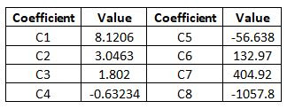
Definitions
Table 2
is a listing of the coefficients. C1, C2, …C32 are alternate references to
these coefficients used elsewhere in the paper. Table 3
lists major variables and GW-BASIC reserved words used.

Table 3 Listing of Important Variables and
GW-BASIC Reserved Words

RESULTS
Optimization of the coefficients in the model used one
hundred and sixty two data points for fitting. The raw information for the data
points was H100, V210 and MW. Testing the model used 40 pairs of randomly
generated V100 and V210 values. The H100 value calculated from V100 and the
V210 viscosity allowed finding the MW from the chart. Table 4
has the statistics comparing the MWC’s to the MW’s for the 2 sets of data along
with ASTM precision data.
Table 4 Model Fit to ASTM D2502 and
Validation Statistics

ASTM D2502-92 (Reapproved 1996) has a 3 g/mole repeatability
(r) and a 25 g/mole reproducibility (R) but it was not obtained in accordance
with R:D02-1007, “Manual on Determining Precision Data for ASTM Methods on
Petroleum Products and Lubricants.” Assuming laboratories received pairs of
viscosity values and they determined the molecular weights, the repeatability (r)
and reproducibility (R) can be calculated from the reported MW’s. The
relationship to the standard deviation (SD) for r and R (Sr and SR)
is assumed to be S= (r or R)/(Z*sqrt(2)) with the Z score of 1.96. The model
has about twice the fit error as the repeatability of reading the chart using
duplicate data by a single person in a single laboratory and 1/4 of the
reproducibility error between laboratories. The calculation is much better for
comparisons between laboratories. The initial fit of 110 data points showed
around 15-20 points with large differences between MW and MWC. Rechecking the
data to eliminate any that were outliers caused by inadvertent estimation and
reading errors showed ten were inaccurate. If this is typical, then 10% of
values determined from the chart will be in error.
The conclusion is the model reasonably estimates the values
from the ASTM D2502 chart. The avoidance of inadvertent estimation errors is a
better trade off as the loss in precision is smaller than the potentially larger
errors during the estimation process. As it will be shown later, the loss in
precision is small compared to the actual variation of the experimental data.
DISCUSSION
Data Modeling and Testing
The initial work used 110 data points selected from the
22x28 inch chart offered by ASTM. Comparing these to the one hundred and three
points reported in the original paper by Hirschler[4] (page 158, Table XI) showed fifty-one
of them to be duplicates. Because the H100 had to be estimated, there were
differences in the H100 values between the duplicate sets with the largest
being 4. For the duplicate data, Hirschler’s data took precedence over the data
read from the chart. This gave one hundred and sixty two data points to
determine the coefficients for the model (fifty-nine taken from the 22x28 inch
chart offered by ASTM and one hundred and three from Hirschler).
These additional points were chosen from the chart to
extended the extremes of the H100 function, to extend the extremes of the
molecular weights, to fill in gaps on the original data (450, 550 and 650
molecular weight) and to included points on the 15 cSt at 210 °F isostoke.
This gave a uniform coverage of the chart. The points chosen are where the H100
lines crossed isostokes of the 210 °F viscosities defined on the
chart. This allowed for a more consistent linear interpolation of the axis
values of the molecular weight, as the spacing between the 210 oF isostokes
is non-linear. These points along with 40 additional test points used to
determine the coefficients in the model are in Figure 1
along with their distributions in Figure 2.


Figure 2 Distribution of MW Data used for
Fitting and Testing ASTM D2502 Model
Modeling
Hirschler’s equation
[1], referenced in his paper as (5), defined the “H” function as a modified
version with 0.6 in place of 0.8 used by Bell and Sharp[5].
Ht
= 870Log (Log (Vt + 0.6)) + 154 [1]
where in [1]
Ht = the “H” function
at temperature t
Vt = the kinematic
viscosity in cSt at temperature t
Log = logarithm to
base 10.
The inverse of the of Ht equation [1] is [2] and referenced
as invHt is
Vt
= 10^(10^((Ht -154)/870))-0.6 [2]
For determining the coefficients for the model, equation [2]
converted Hirschler’s data and the chart H100 data to V100. V100 is one of the
inputs for the model.
Equation [3], given by Hirschler as (6), to calculate the
molecular weight of an oil
MW
= 180 + S(H100 + 60) [3]
where
S =
4.146-1.733Log(VSF - 145) [4]
VSF=H100-H210 [5]
and VSF is the viscosity slope factor as defined by Bell and
Sharp5.
Through simple algebraic substitution and rearrangement,
equations [1], [3], [4] and [5], the MW calculation reduces to the form of [6]
MW = [180+4.146(154 + 60)] + [4.146*870]*F1
+ [-1.733*870]*F1*F12
+ [-1.733 (154+60)]*F12 [6]
and generalized to [7]
MW=
C5+C6*F1+C7*F1*F12+C8*F12 [7]
where
F1=Log(Log
(V1+C1)) [8]
F2=Log(Log(V2+C2)) [9]
F12=Log(F1-C3*F2-C4) [10]
C1
to C8 = Coefficients.
Although Hirschler’s paper used log to the base 10, the fit
in GW-BASIC uses Log to the base e. There is no issue in replacing Log base 10 with
log base e (Ln) as they are linearly related by a constant (Log=2.3025*Ln). References
to a Hirschler model in this paper denotes equation [7] using Ln.
Using the initial 110 data points from the chart before the
Hirschler data was available from his paper gave the statistics in Table 6
and the C1 to C8 coefficients in Table 5.
A self-written nonlinear least square (NLLSQ) program written in GW-BASIC[6]
determined the coefficients. After entering a set of initial guesses for the
coefficients, the program used a sequential simplex[7] to
modify the coefficients to find a minimum residual sum of the squares. Eventually,
a set of initial guesses led to a set of “optimized” coefficients, where no other
set of initial guesses seemed to lead to a set of coefficients with a lower
residual sum of squares.
Although, the coefficient set yielded a model with good
regression statistics (Table
5)
the standard deviation for the residuals were higher than desired.

Table 6 Hirschler Model Coefficients
Figure
3 is a plot of the residuals (MW-MWC) from fitting the
coefficients using Lotus[8] 1-2-3
with residual value as data labels. Lines of constant residuals are hand drawn.
The negative values indicate the MWC was higher than the MW from the chart. The
negative residuals delineate a “peak” or area of higher observed values at the
coordinate at MW=400 and H100=400, 600 and a “valley” or area of low observed
values at MW=600 and H100=500 with somewhat elliptical contours. Figure 4 is the same plot as Figure
3 but updated to include all 162 fit data points. It
confirms the original contour plot.


To find an improvement to the fit, higher polynomial terms
for F1, F2 and F12 were added to the initial Hirschler model. All 34 (combinations
with replication) of the first through the fourth order terms and second through
fourth order cross function terms of F1, F2 and F12 (i. e. (F12, (F1)^2, (F1)^4,
(F12)^2*(F1)*(F2), (F12)*(F1)*(F2), (F1)^2*F3^3 etc...) were generated. An
online computational service[9] with
access to a stepwise multiple linear regression program[10] was
used to select the most significant terms for inclusion in the model based on r2
and F-ratio. Equation [11] and the calculation algorithm line (d) shows the
terms chosen and used in the model.
MW=C5+C6*F12+C7*F12*F2^2+C8*F1^4+C9*F1*F2*F12 [11]
This model has a residual
pattern similar to Figure
3 so it was further modified to include corrections for
the high and low residual areas. Since the residual areas appeared elliptic, skewed
and only local deviations needed modeled, a normal distribution was used to
model each area. The modification to the normal distribution included
translation from the origin, rotation of the axis, making it pseudo-bivariate with
elliptic contours and skewing of the distribution. Calculation lines (g)
through (s) and (t) through (af) are these modifications. A more detailed
explanation of the modifications is in the MODEL AND CALCULATION DETAILS below.
The 2 corrections, MW1 (s) and MW2 (af), are added to the initially calculated
molecular weight MW0 along with the bias coefficient C(32) to give the final
molecular weight MWC (ag).
Coefficients
The model fit in GW-BASIC used double precision calculations.
This calculation gave the coefficients 15 significant digits, an amount that
would be tedious to use and masked any calculation sensitivity. The number of significant
digits was reduced for each coefficient until any calculated molecular weights changed
by 0.1. That digit was then added back with rounding to the coefficient. The
sum of the square for the single and double precision sets of coefficients was
867. Table 7
lists the coefficients.

Results
Figure 5
shows the calculated V210 isostokes from the fitted model along with the data
points from the ASTM chart.

Along with Data
Points from ASTM Chart
Table 8
is the statistical information or the final fit.
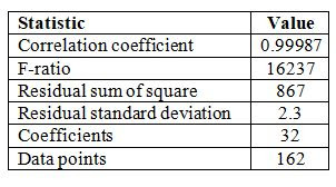
Figure 6,
Figure 7
and Figure 8
are the corresponding line plot, residual distribution and residual normal
probability plot respectively.

Figure 6 Line Plot of ASTM D2502 Model Fit

Figure 7 Residuals from ASTM D2502 Model Fit

Figure 8 Normal Probability Plot of Residuals
from the Model Fit to ASTM D2502
Figure 9
plots the data points labeled with the residual (MW-MWC) from the fit. Points
that have a residual >±4
are highlighted in a white circle. These are clustered on the right edge and
upper right corner. A recent recalculating the results in Excel using the
original data and the reduced precision coefficients verified the model. The Excel VBA code for the calculation is at the
end of the paper.

Figure 9 Final Fit Residuals ASTM D2502
The figures 5 through 9 show how well the model represents
the chart.
There were no distinct patterns in the residuals when
plotted against the independent input viscosities. There did seem to be a
possible “rocket nozzle” like pattern for the residuals versus the MW. The
variation in the residuals was slightly wider at low MW’s and even wider at
higher MW’s. This may suggest a transform of the MW may be useful or it could
be an artifact that the curves drawn by Hirschler are more variable in their
placement because the low and high MW areas have little or no experiment data
to estimate the curve drawing. Additional work later in this paper fitting MW and
MWE to the viscosity data using Table Curve 3D[11]
shows many of the fits used an inverse or Ln transform of the molecular weight.
Figure 10
shows the pattern.

Figure 10 Model Fit Residuals Pattern with MW
Experimental Data
Review
Hirschler’s paper4 examined available data from 9 sources and
chose what he considered the most reliable results and gave that data
“paramount consideration” when designing the chart. These are the reference 26,
27 and 24 with the same major author, same molecular weight determination
method and same oil but somewhat different extraction, distillation and
hydrogenation treatments. This will bias them to be similar but also lends
itself to comparing the molecular weight data with samples of similar viscosities.
The ASTM chart is a modification of a chart in reference 18 page 462. The chart
in this reference has straight isostoke lines and Hirschler considered the
correlation inaccurate. Table 9
lists the references and comments about them. The comments in italics are this
paper’s author. One issue that adds more variability beyond the variability
between the molecular weight methods and viscosity instrument accuracy is the
conversion of SUS[12] to cSt by Hirschler and
this paper’s author. References 9 and 10 has SUS viscosities listed in SUS and
cSt that did not convert using ASTM D2161-93 Reapproved 1992)є2.

There were 233 experimental points. Only 217 are in the area
covered by the chart. Sixteen from reference 12 have H100’s or MWE’s too low to
be put on the chart. Figure
11 shows the distribution of all the experimental data
with labels from Table 9
indicating the Hirschler reference. The point “a” at MWE=172.5 and H100=230.2 is
considered suspect (see Erratum). Figure
12 displays the experimental data covered by the same
area as in the ASTM chart. Data labeled 2, 3 and 4 are from references 26, 27,
and 24 and were the ones given the most weight by Hirschler. It is evident from
Figure 12 that the ASTM chart has sparse experimental data in
the lower and upper right quadrants. There is also limited data below a 250
MWE.

Figure 11 Experimental Data Figure

Figure 12 Experimental Data with ASTM D2502 Chart Limits
Figure 13
has the experimental points color coded to emphasize the methods used to
determine the molecular weights. Figure 14
is similar for viscosity methods. The color-coding is to show visually any area
that might have a data bias based on methods. The methods are distributed
across the chart.

Figure 13 Experimental Data MW Method

Figure 14 Experimental Data Viscosity Method
The relationship of the 2 viscosities for the experimental
samples is shown in Figure 15
and the distribution of the determined MWE is in Figure 16.
The MWE centers on a 400 MW.

Figure 15 Viscosities of Experimental Samples

Figure 16 Distribution of Molecular Weights
(MWE) for Experimental Samples
The format of the ASTM chart and a plot of the raw
viscosities can mask the high degree of collinearity of the viscosities that is
more evident when the viscosities are plotted as H functions as in Figure 17.
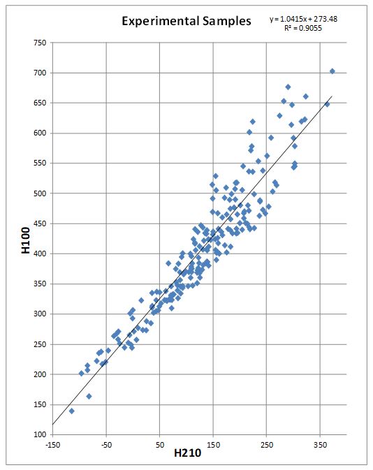
Figure 17 Experimental Samples Viscosities Collinearity
When the axes ranges are limited to the central area in Figure 17,
the MWE labels are less cluttered and more readable (Figure 18).
Figure 18
begins to hint of a molecular weight trend perpendicular to the relationship of
H100 to H210.

Figure 18 Experimental Samples Molecular
Weights
Experimental Best Case (MWE) vs. the Chart (MW)
The purpose of reviewing the experimental data is to
understand how well it compares to the ASTM chart.
Table 10
has 25 experimental points (MWE) selected from the set of 86 points in references
24, 26 and 27. The 86 points are from those given “paramount importance” by
Hirschler. This subset of the total experimental data (214 from 9 references) is
a best-case comparison of the data to the chart. Table 10
also has the corresponding molecular weight data from the chart (MW) and chart
model (MWC) as well as the differences between the various molecular weights.
The comparison of
the chart and calculated MW’s (MW-MWC) has a SD of 3.6. This is higher than the
2.1 in Table 4 found during the fitting of the model to the
chart. The points selected for fitting the model were on the well defined integer
crossing points of the H100 and the V210 line. Only the MW needed
interpolation. For the experimental data, the H100 and viscosity were
non-integer and required estimating where the point was on the chart. The
higher SD of this data reflects this and supports the problem outlined in the
INTRODUCTION.
Table 10
shows, expectedly, that the chart and calculation (MW-MWC) are in better
agreement than the MWE-MW and MWE-MWC differences. The SD for this best case is
better than the SD’s (22, 27) in Table 13,
which is fitting the model to the experimental data. This supports that the
chart is biased toward the data in the first 3 references.

The correlation of the molecular weight data in Table 11
exemplifies that the chart and model are more closely related than they are to
the experimental data. The relationship of the chart and model to the
experimental data is similar. The regression plot in Figure 19 is a plot of the experiment molecular weight and
chart data in Table
10. The regression has a slope of 0.99±0.03 and an intercept of
9±14 and affirms the relationship of the experimental data to the chart. Figure 20 is the pattern of the experimental points for the data in Table 10. Since the pattern covers most of the chart, it is
not biased to any region.


Figure 20 MWE-MW Differences for Data and Chart
in ASTM D2502
Model Predictions
A complete comparison of the difference between the MWE’s
and MWC’s are in the data Table 35
at the end of the paper. The precision of the raw data listed in the table is
that from the references. Graphically the differences are shown as point labels
in Figure 21.

Table
12 compares the molecular weights calculated (MWC) from
the experimental viscosity data using the method in this paper and the
experimentally determined molecular weights (MWE) for each of the Hirschler
references. The model fit has repeatability worse than reading the chart (6 vs.
3). Its reproducibility is much better (6 vs. 25). The model and the chart are
equal in representing the experimental data. A model should not be more precise
than the experimental data. In this case the model is better than the data
because the idealized chart is modeled and not the data. The standard
deviations for the model fit to references 24, 26 and 27 are about one-half to one-third
the other data sources. The experimental data is likely more consistent for
these references as they are by the same main author, on similar oils using the
same molecular weight method and Hirschler gave them more importance in making
the chart.
Table 12 (1 of 2) Details of Molecular Weight Model
Fit to Data from Hirschler,
ASTM D2502 Chart and Experimental Results

Table 12 (2 of 2) Details of Molecular
Weight Model Fit to Data from Hirschler,
ASTM D2502 Chart and Experimental
Results

Determining the best coefficients to fit the model to the 214
experimental data points (excluding data in reference 12) showed major shifts
in them that would indicate a much better local or global optimum for the
experimental data was possible. It did reduce the sum of the squares but there
was only a moderate change in the standard deviation of the residuals. Expectedly
with the refit, the minimum residual became more negative and the maximum
became less positive for the refitted model. The average of the residuals
became close to zero as would be expected. Residuals for a good model fit have
a normal distribution centered on zero.
Table 13 Residuals for Fitting Model
Coefficients to Experimental Data

Whether there would be value in attempting to model actual
experimental determined molecular weights to get a better model fit would
depend on the variation of the MWE’s.
Variation of Experimental Molecular Weight (MWE) Data
Using a cluster analysis of the samples’ viscosities to
determine which ones were most similar, gave those listed in Table 15.
Those selected for this list would depend on the clustering method, how to
define the “same” viscosity and the precision of the viscosities and molecular
weight determinations.
There are many forms of cluster analysis. Points visually close
to each other were selected from a chart of H100, MWE and V210 isostokes. These
were compared to a cluster analysis using Euclidean distance measurement with
single linkage amalgamation. The visual proximity of a single pair of points
did not match the cluster amalgamation. The discrepancy seemed related to using
the linearization V100 (H100) versus the non-linear nature of the V210 lines. After
conversion of the viscosity data to F1 and F2 functions that are analogous to
the H100 and H210 function, the cluster analysis gave samples more reasonably
similar for both viscosities. The F1 and F2 functions used were the Ln Ln of
the corresponding viscosity and its corresponding coefficient from the model (as
exampled in calculations (a) and (b)).
The second item
is determining the “same” viscosities. ASTM D445 has a repeatability of 0.0011%
of the sample’s viscosity for base oils at both viscosity temperatures. If the
viscosities fall within the repeatability then they are not considered
different.
The initial
thrust was to find a set of similar samples from the same reference and a set
from different references to get some understanding of the impact of the
analytical methods and reproducibility between laboratories. The data analyzed
consisted of only amalgamated sample pairs. There were no triplicate or higher
amalgamations used. Using the ASTM repeatability gave no set of samples where
both viscosities would be the “same”. To get a minimum of 5 samples preferably
for both sets of samples (same and different references), the repeatability
range was widened. It was not possible to get at least 5 samples for each set.
The closest 10
pairs of samples are in Table 15.
Calculations include values that give the range of molecular weights for the
sample pairs using their maximum and minimum viscosities. The molecular weight with
the maximum V100 and minimum V210 would give the lowest MWC while the minimum
V210 and maximum V100 would give the highest.
Table 14
shows the comparison of the standard deviations (SDs) for selected sample pairs
and that of the MWC. Not included were those having large percent differences
in V100 unless they were from the same reference. Sample pair 5 had a V100
difference of 1.9% yet the molecular weight difference was only 1.0. One would
expect the molecular weight difference to be more if the molecular weight
analysis and correlation of viscosities to molecular weights are reliable. The difference
in standard deviation for sample pairs from different sources, which could also
include different molecular weight methods, compared to the standard deviation for
sample pairs from the same reference was extreme at 22 vs. 1.4.

Table 15 Experimental Samples with Similar
Viscosities

Comparison
ASTM D445 Viscosity Measurements
Viscosity measurements will affect the calculated oil’s
molecular weight. This is not a rigorous attempt at the propagation of error.
The repeatability and reproducibility of the method for base
oils given in ASTM D445 is in Table 16.
Both values are a percent (0.0011 = 0.11%) of the measured value. The measured
value is x in Table 16.
The precision values for base oils are the lowest for the types of oils listed
in the method so represent a best-case scenario.
Table 16 ASTM D445 Percent Repeatability and
Reproducibility for Base Oils

Three H100 values were chosen that represent the bottom,
middle and top of the chart (100, 400 and 620). These represent viscosities of
6.759, 82.18 and 2707.5. Eight V210 viscosities that intersected the V100
viscosities were selected; two for the bottom, three for the middle and three
for the top. Table 17
has the repeatability and Table 18
has the reproducibility. The viscosity values highlighted in yellow are in
pairs with the second in the pair having the repeatability or reproducibility
value added.
For a given V100, a higher V210 viscosity will give a higher
MWC. For a given V210, a higher V100 viscosity will give a lower the MWC. Given
a set of high and low viscosities for both V100 and V210, the maximum MWC for
this set is when the low V100 and high V210 are used. The minimum is when the
high V100 and low V210 are used. Table 19
illustrates this.
The SD for the Max-Min. of the reproducibility is 1.8. As it
is unlikely that both measurements would be at extreme values, the more
reasonable value 1.4 = (0.6^2+1.3^2)^0.5 will be used for comparison. The SD
for the model fit is 2.3 (Table
4).
The variation in the viscosity measurement can approach 60-80% of the model fit.


Table 19 MWC Max-Min. Relation to Viscosities

Maroto and de las Nieves[14]
This paper details a refinement in the molecular weight
calculation by Hirschler where a cubic polynomial of the VSF function replaces the
S function in equation [4].
Doing the various algebraic substitutions led to the
generalized equation for MWC of [12].
MWC=a+bη4+cη3+dη2+eη+fηH+gηH2+hηH3+iη2H+jη2H2+kη3H+lH+mH2+oH3 [12]
where
Table 20 Coefficients of the
Generalized Calculation in the Maroto Paper

The Maroto paper used the H function with the
standard j, k and l coefficients. In this paper, the H functions were a
generalized version at 100oF and 210oF referred to as F1
and F2 where the H function coefficients were optimizable parameters. The S
function has a Log function of the VSF. Using the cubic modification of the VSF
for S, there is no longer a Log function of the VSF. In this paper, keeping the
Log function of the VSF causes the generation of the F12 function, which is a Log
function of the combined F1 and F2. There is no corresponding H12 in the Hirschler-Maroto equations.
A matrix of the 14 terms in equation [12] shows the powers
(order) of the H100 function, the H210 function and the
cross-product terms (X’s).
Table 21 Matrix of Terms in the Hirschler-Maroto Model

Table 22
shows a comparison of the H or F polynomials used in the calculations in this
paper and in the Maroto paper. The 3 tuples in the table indicate the power
of the cross-term functions. The tuple 0,2,1 represents F10*F22*F121.
The Hirschler-Maroto equations have more polynomial terms than the calculation in this
paper. However, the elliptic and skewed normal functions required 22
coefficients (11 for each of the 2 elliptics) for modeling areas of the
residuals but it also resulted in modeling a much wider area of the chart.

What
was interesting about the Maroto paper was how the area of the results
compared to the actual experimental data. Figure 22 has the experimental data shown in Figure 12 bounded by an irregular decagon. The area centered on the H100=590 and
Relative Molecular Mass=380 area are points from Hirschler reference 26 which
he considered “paramount”. In Figure 12, these points have the label 2. The Maroto modification does not model
this area of the ASTM chart.

Figure 22 Hirschler Experiment Data Outlined on
the Restricted Maroto Chart
(Fig. 3. in their paper)
Criticisms
ASTM
This calculation was presented to C. L. Stuckey chairman of
ASTM Committee D02.04 in 1991. At the June meeting, Rinus Daane of Shell
Research, Europe commented that:
1.
The data was a mix of actual and
artificial data, and a correlation of a correlation.
2.
Thirty-two coefficients did not
qualify as a good correlation and was “hocus pocus.”[15]
3.
The viscosities were non-standard
and not at the standard temperatures of 40oC and 100oC.
He recommended leave the method as
is or develop a new correlation.
In response,
1.
The data for the fit was not a mix
of actual and artificial data. Hirschler gave data in his paper to generate the
chart. The calculation used the idealized data from his paper and additional
data points were taken from the chart. All the data was of the same type.
2.
Thirty-two coefficients would
normally be a lot if the calculations were simply using higher order
polynomials that generate small differences to make the fit better. They also
start to model noise. If this was the reason for the polynomials, I would agree
it is “hocus pocus.” However, the polynomials showed significance in the Stat
II fits. Because the polynomials were significant and the coefficients needed
only a limited number of significant digits, I do not believe they represent an
example of Runge's phenomenon[16]
or the modeling of noise.
3. There was no intent for it to be a replacement with new
experimental data or methods but only to model the chart. This work was to
avoid the inconvenience and errors of interpolating data from the chart. The
work showed that about 10% of the molecular weights read from the chart would
be in error. Other ASTM methods have both a chart or table and a calculation
associated with them. By example, ASTM D341 has a calculation with 13
coefficients.
Incorporating the calculation into
the method was due to the lack of a task force leader that could devote the
time needed for the project.
Hydrocarbon Processing
Hydrocarbon Processing rejected the manuscript on
calculation of molecular weight because it did not meet their editorial needs
at that time (12/12/1985).
Concerns
The only concerns are the molecular weight transition for
the EL1 and EL2 elliptic skewed normal distribution sign change. For the EL1,
the transitions are modest being less than 5. The transitions for EL2 are much
larger but are in areas that are on the extreme edge of the chart where there were
no real samples. The section Elliptic
Transition with Skewed Normal Distribution discusses this and is shown in Figure 27 and Figure 29.
MODEL AND CALCULATION DETAILS
Model Background
The purpose of the NLLSQ program was to become familiar with
the modified sequential simplex optimization method and use it to develop
formulation mixtures. It would also provide a flexible least squares fitting program
for use on other laboratory data. It proved inappropriate for mixtures because
of the formulation constraint in that type of design of experiment (DOE[17]).
The misuse of sequential simplex for mixture designs are in the literature[18]. The
fitting of a model to the ASTM D2502 chart was a method to test the program and
possibly avoid the inconvenience of reading the chart.
Hirschler Model F1, F2, F12
F12’ equation [13] is a term used in the Hirschler model equation
[7] before it was generalized. The following steps detail how F12’ was
generalized to F12. It also shows how the functions and coefficient from the
generalization manifested themselves in the higher order function polynomials
of equation [11].
F12’ Generalization
F12'=Log(870*F1-870*F2-145) [13]
Algebraic manipulation of [13] yielded [15].
F12'=Log(870*(F1-1*F2-145/870)) [14]
F12'=Log(870)
+ Log(F1-1*F2-145/870) [15]
The “1” before F2
and the constant 145/870 were generalized by making them C3 and C4 shown in
equation [16].
F12'=Log(870)
+ Log(F1-C3*F2-C4) [16]
The use of F12 simply means the C5 constant in equation [11]
will include the constant Log(870) from equation [16].
F1*F12 Generalization and Reduction
For the C7*F1*F12 term from equation [7], the generalization
of F12’ [16] will generate a second F1 term in equation [18]
C7'*F1*F12=C7'*F1*[F12'-Log(870)] [17]
C7'*F1*F12=C7'*F1*F12'
-C7'*F1*Log(870)] [18]
The C6
coefficient in equation [20] for F1 would essentially be a combination of other
coefficients and constants of the non-generalized form of F12.
C6*F1=
-C7'*Log(870)*F1+C6'*F1 [19]
C6*F1=
(-C7'*Log(870)+C6')*F1 [20]
Model Elliptics + Skewed Normal Distribution Adjustments
The residuals from fitting the Hirschler model have a pattern
of a high “peak” and of a low “valley” area seen in Figure 3. It seemed that the 2 areas could be modeled by 2 modified
normal distributions, a positive and a negated one. They would have a structure
where the value at farther distances from the center of the high or low area
would go to zero and just be adding correction terms to the initially
calculated molecular weight (MW0). The areas also looked possibly elliptic and
possibly skewed on the various sides of an elliptic axes. A calculated elliptic
contour became the basis of a normal distribution creating a bivariate-like
normal distribution from a univariate distribution. Replacing the typical
quadratic power of e with a quartic order polynomial introduced skewing. In
crossing the axes, the X value would become negative. Expecting the sign change
would cause a possible jump in the value from the distribution, the negative X
values were converted to positive values when the axes were crossed. The
calculation used two elliptics, EL1 (m) and EL2 (z).
Elliptics
The axes of the ASTM chart are MW and H100. The translation
and rotation of the elliptics used the axes of MW0 and F2. Since MW is being calculated,
it is not available as data to translate and rotate the axes. Residual contours
of H210 and MW were similar to the contour using H100 but appear more uniform
so the generalized F2 function was used.
Translation and rotation of a function in Cartesian
coordinates from (0, 0) origin to a new origin at (X,Y) are shown in equations
[21] and [22][19].
X = (x − h) cosθ + (y − k) sinθ
= x*cosθ + y*sinθ - h*cosθ - k*sinθ [21]
Y = − (x − h) sinθ + (y − k)
cosθ = y*cosθ - k*cosθ - x*sinθ + h*sinθ [22]
Expansion of
Equations [21] and [22] with the replacement of X with MWS and Y with F2 gives
equations [23] and [24]
X=MWS*CO1+F2*SI1-C(11)*CO1-C(12)*SI1 [23]
Y=F2*CO1-C(12)*CO1-MWS*SI1+C(11)*SI1 [24]
where
X = the translated and rotated
coordinate in terms of MWS (x-axis)
Y = the translated and rotated coordinate
in terms of F2 (y-axis) – note not F1
MWS = the scaled primary molecular
weight MW0 in calculation (e).
SI1 = SIN(C(10))= sine of the
rotation angle of the first ellipse
CO1 = COS(C(10))= cosine of the
rotation angle of the first ellipse
C(10) = angle of rotation (θ) of the
first ellipse determined by regression
C(11) = translation in the x axis (h)
determined by regression
C(12) = translation in the y axis (k)
determined by regression

Figure 23 Translation of the Origin and
Rotation of Axis with Elliptical Contour
Equation [25] shows the standard elliptical.
X2/b2+Y2/a2=1 [25]
Since equations [23] and
[24] have the translation and rotation incorporated, there was no need to do
the translation to the center point of the ellipse or its rotation. The new
origin coordinates (X, Y at point OT) were divided by regression determinable
coefficients C(13) and C(14) making them equivalent to equations [26] and [27].
X/b=X/(C(13) [26]
Y/a=Y/(C(14) [27]
Combining [23] with [26] and
[24] with [27] gives the form of the calculations for the elliptics.
Calculations (i) and (k) shows these the elliptic contour forms EL1 (v) and EL2
(x).
X1 and Y1 were then squared
(calculations (j) X12 and (l) Y12) and added together (calculation (m)
EL1=X12+Y12) to make an elliptic contour defined as EL1. EL2 used the same
calculations but with other coefficients.
A normal distribution used
the elliptic contour values to calculate the adjustment in the initially calculated
molecular weight (MW0). Equation [33] shows a generalized normal distribution
(GND). The modified generalized normal distribution (MGND) equation [35] was
the GND altered by having Euler’s e raised to the 4th power
of the elliptic contours EX1 or EX2. An issue might occur if the distribution did
not have a smooth transition across the elliptic axis and result in jumps in
values when the point was on one side of the axis or because of the odd terms
in the distribution. Changing the signs of the elliptic values on opposite
sides of the axes made them consistent. Using them in the higher order polynomial
normal distribution, the coefficients would regress to the appropriate negative
or positive values. If the calculation in equation (n) indicated the EL1
(ellipse 1) in equation (m) was negative, it was made positive by multiplying
by -1 in equation (p) (EX1, exponent 1).


In the calculation, the
coordinates of the center of the ellipse was defined by the coefficients
(C(11), C((12)) and the point P1 by the coordinates (MWS,F2). To determine
which side of the rotated and translated ellipse a point was on, the coordinates
of the point would be used to calculate the angle of the point from the original
axes. Figure 24
visualizes putting the center or origin of the ellipse, point OT (origin
translated) in Figure 23,
superimposed on the original origin. Angle ϕ of the point would be compared to
θ, the angle of the rotation of the ellipse (C(10) for ellipse 1). If ϕ> θ
or (Tanϕ>Tanθ), it would be considered on one side of the axis. Otherwise,
its sign is changed. Tanϕ is the length of H/length of D. In terms of the
coordinates of the 2 points (P1 and O) and the coefficients in the model, equation
[28] defines Tanϕ.
Tanϕ=(F2-C(12))/(MWS-C(11)) [28]
We are looking
for
Tanϕ>Tanθ [29]
Substituting in
equation [28] and the tan of the axis rotation, Tan(C(10))
(F2-C(12))/(MWS-C(11))>Tan(C(10)) [30]
0>Tan(C(10))*(MWS-C(11))+C(12)
-F2 [31]
gives equation [31] which is
the form of calculation (n) and (aa) to SG1 and SG2. The algebraic manipulation
rules for the multiplication or division of an inequality were not necessary, as
the absolute value of the sign is not important. For the calculation, it is
only important to know if they are on the same side of the axis and if they are
not then the sign is made the same. Figure
25 uses the tangent calculation equation to determine
the sign on either side of an ellipse axis. The x and y values are
representative data. The labels on the axes and title are the actual data name
or calculated intermediate used in making the model but are appended with an
apostrophe (’) to indicate the use of representative data in making the figure.
Skewed Normal Distribution
Starting with a normal distribution equation [32],
generalizing to give the generalized normal distribution (GND) [33] by
consolidating constants and expanding the exponential term, and then replacing
the exponential term with a higher order polynomial [34] gave a modified
generalized normal distribution (MGND) equation [35]. Recent literature has
referred to this as a flexible skew-symmetric distribution[20], [21], [22], [23].
GND=ae-(b+cX+dX^2) [33]
(b+cX+dX2+eX3+fX4) [34]
MGND=ae-(b+cX+dX^2+eX^3+fX^4) [35]
X in equation [35] represents EX1 in calculation (p) and EX2
in calculation (ac). The polynomial [34] is written in the Horner[24] nested
polynomial format to avoid generating large numbers with the higher
polynomials. It was also broken into parts for easier coding and represented by
calculation (q), (r), and part of (s) and calculations (ad), (ae) and part of (af)
for the 2 elliptic skewed normal distribution adjustments. Calculations (s) and
(af) yield the elliptic skewed normal distribution adjustments to the molecular
weight. Equation 36 represents the full function calculation of adjustment 1
with the coefficients being represented without the array parenthesis.
MW1=C15e^(-(C16+C17*EX1+C18*EX12+C19*EX13+C20*EX14) [36]
Figure 26
shows some of the various forms that can be generated by higher order
polynomials in a normal distribution and Table 23
has some description details with the coefficients used to generate the curves.

Figure 26 Examples of Higher Order Normal
Distributions
and the Coefficients of the Powers of X

The “a” through “f” coefficients in Table 23
are those in equation [35]. EX1 and EX2 are the ellipses from the fit. They
were both negative. A rescaling of EX1 and EX2 allowed plotting them in Figure 26.
EX1 has a small minimum so rescaled larger. EX2 was massively larger and
rescaled considerably smaller to fit on the chart. There is a considerable
range of forms for the residuals that adjusting these terms could model.
A second skewed normal distribution calculated (calculations
(aa) through (af)) in the same manner as done for the first. This generated a
second molecular weight adjustment (MW2)
The base molecular weight MW0, MW1 from the first elliptic
and skewed normal distribution and MW2 from the second elliptic and skewed
normal distribution are combined to get the final calculated molecular weight
(MWC).
Elliptic Transition with Skewed Normal Distribution
One of the
concerns was how well this would work. No transition issues were apparent when
originally investigated. In preparing the graphic visualization of the
transition lines with more granular inputs, they appeared.
Figure 27 to Figure 30 shows the sign transition for both ellipses. The
first chart of each pair uses the same axes (H100, MW) as the ASTM chart while
the second has axes based on the calculation parameter used for the ellipses
(F2, MW0). The use of F2 causes the curved transition lines in Figure 27, Figure
29 and Figure 33.
All the figures show smooth transitions but the granularity is the size of the data
point on the plot.

Figure 27 Ellipse 1 Sign Transition

Figure 28 Ellipse 1 Sign Transition

Figure 29 Ellipse 2 Sign Transition

A granularity of
<0.05 for the H100 function showed the transition.
Figure 31 and Figure
32 show the magnitude of the effect for EL1 and EL2. Table 24
lists the values for EL1 and EL2 at various V210’s. For EL1 the maximum amount
is 5 at a V210 of 6 and for EL2 is a maximum of 15 at a V210 of 60. Figure 33
shows the transition for the experimental data. The EL2 transitions are
essential in an area devoid of any experimental data and would have a low
likelihood of being encountered in practice (Figure 33).
The EL1 transition is in an area where there is experimental data close to the
middle of the data. Although the amount is higher than desired to match the repeatability
of reading the ASTM chart, it is within the reproducibility and similar to the
difference seen with experimental samples.


Figure 33 Elliptic Transitions with
Experimental Data
Coefficients Purposes
The coefficients are color-coded indicating their use in the
calculation.
Table 25 Coefficients Color-Coded by
Function in the Calculation

Table 26
Explanation of Model Coefficients

Viscosity Conversion
Some of the viscosity data in the references is SUS. For use
in the calculation, they had to be converted to cSt. The calculation {1} of the
SUS from cSt at a temperature T used the formula given in ASTM D2161-93
(Reapproved 1992)є2 page 2 Equation (6). This equation was used to
convert SUS data reported in the references to cSt for input to the model.
SUS
is calculation is cell A1
=
(1+0.000061*(C1-100))*(4.6324*B1+(1+0.03264*B1)/((3930.2+262.7*B1+23.97*B1^2+1.646*B1^3)*0.00001)) {1}
where
the cell references in {1} are defined in Table 27.
Table 27 Cell Content for Calculation SUS from
cSt

Some references with viscosity and molecular weight data reported
both SUS and cSt viscosity values. Using {1} did not give the same cSt
reported. A reverse calculation from cSt to SUS was used to further compare the
2 reported viscosities. Previously a method for doing the reverse (InvSUS) calculation
had been developed. It is detailed in the Calculation Codes section. Since it
was available, the cSts reported were converted to SUS and reaffirmed the
values did not convert equivalently using the current calculation. This adds
another element of variability in the experimental data as all of the
references that used SUS and converted for use by Hirschler or the reference’s
authors may not be consistent with the current conversion method.
REVELATIONS
Experimental Data MW Trends
The MWE data follows trends. It increases from samples that
have low values of H100 and H210 to those that have high values as shown in Figure 34.
This is not a surprising trend, as higher molecular oils would generally have
higher viscosities and give higher H functions for both. In Figure 34,
the MWE’s have only their first digit plotted to make the chart readable. The
MWE’s vary from 250 to 450 along the dotted regression line of H100 and H210.

Figure 34 Experiment Molecular Weight Trend
Related to H Functions

Figure 35 Variation of the Average Molecular
Weight along the Regression Line
In addition to this trend, a trend of decreasing molecular
weights perpendicular to the H100 and H210 regression line is discernible in Figure 34.
Figure 36
using MWE/100 data labels and Figure 37
using data points show the data and trend more clearly. The reason for choosing
lines perpendicular to the H100 and H210 regression line was arbitrary based on
the appearance of the molecular weights on either side of the trend line. Figure 36
and Figure 37
have points chosen close to several perpendicular lines by calculating the
distance from the experiment points to a specific perpendicular line and
selecting a subset of the closest ones.

Figure 36 Experiment Molecular Weight Trends
Perpendicular to the
H100 and H210 Regression Line

Figure 37 MWE Data Point Proximity to
Perpendicular Lines
Other Approaches
The near linear components of the 2 trends in Figure 34
and Figure 37
suggested that other approaches may have interest for both fitting the data to
the ASTM chart (MW) and to MWE. These would include:
1. Principal
Component Analysis (PCA)
2. Fitting
a function to the H100 and H210 relationship and then fitting a function
perpendicular to that trend
3. Do
the same as described in 2. but in the reverse order
4. Multiple
Linear Regression (MLR)
5. Fitting
the data with a 3D fitting program like Table Curve 3 D.
PCA selects perpendicular principle components although
there might be some variant that fits non-perpendicular components. This was
the reason for suggestions 2. and 3. as they could include a parameter to vary
the angle off the perpendicular of the lines crossing the molecular weight
trend of the H100 and H210 regression line. Some of these approaches may be
degenerate and lead to essentially similar types of fits.
MLR and Table Curve 3D
The data H100 as x, H210 as y and either MW or MWE as z was
fit to equations using Statistica and Table Curve 3D. These programs report the
standard deviation of the fit as the standard error of estimate.
The equation fits of MWE in Table 30
named MLR 1 from Statistica and Best 3 from TC3D had standard deviations (23,
26) similar to the standard deviation of nearly replicate experimental data given
in Table 14
(22) indicating that there are unlikely to be any models that will fit the
actual experimental data better. Figure 38
is a plot of the TC3D fit Simple 4 and Figure 39
is a plot of the residuals for the Simple 4 fit. They give a visual
representation showing how difficult it would be to find a better model due to
the points being about equally above and the surface of the fitted plane and
being nearly uniformly scattered across it. One of the data points that is
considered a possible outlier is clearly evident in Figure 38
as a red dot with a long red line to the equation plane. The residuals plot in Figure 39
shows a second possible suspected outlier. The circles represent the data
points with the fill colors representing the size of standard deviation. The
color of the lines from the point to the fit plane and the point border color indicates
whether it is above or below the plane. Table 28
is a description of the color-coding used in Figures 38 to 40.

For the Statistica data, the standard deviation of fits to
MWE and MW appear odd in that the standard deviation for the MW is greater than
for the experimental data. The MW data covers a wider area and is not as linear
as the MWE data making the error in a simple linear fit to the chart data greater.
For the best TC3D fits (Best 3 of MWE and Best 6 of MW),
there is a significant reduction in the standard deviation fit for the MW data.
A feature of the Chebyshev[26] polynomial
is it generates a smooth and continuous curve. The bivariate form makes a
surface. Figure 40
plots Best 6 for the MW data as a visual representation that the data points lay
on the smooth continuous equation plane. Because of the smooth and continuous
fit, a better fit to the MW data is unlikely. The same is true for the
Chebyshev fit to MWE. As typically seen with extrapolated empirical fits, areas
outside the fit may not realistically represent data in those areas. The
Chebyshev fit has a “wall” plane on the right of Figure 40
that would not represent any experimental data in that area. The standard
deviation (1.7) for the fit Best 6 was very close to the standard deviation for
the fit model in this paper (2.3 Table 8).
The “Best” equations and the “Simple” equations are considered limiting cases
showing the range of standard deviations for the 2 sets of data.
The Chebyshev Bivariate Polynomial Order 10 is more complex to implement, has 66 coefficients and each coefficient will need at least 6 significant digits (precision) for calculations. Table Curve does not appear to check each coefficient for needed precision but reduces all of them equally starting at 18. The coefficient precision data in Table 29 shows that 6 digits will give a maximum error less than the ASTM repeatability error (Table 4). Coefficients with the next lower precision (5) are significantly worse.
Table Curve 3D has the ability to generate code for the
fitted equations. The inputs for the code are the H100 and H210 values of V100
and V210. Code is available for C 64 bit, C 80 bit, Pascal, Basic, Fortran 77,
Fortran 90, Java, Matlab and C++ from the author.
The Chebyshev
Bivariate 10th Order Polynomial C++ code is at the end of the
paper.

Table 30 Table Curve 3D Equation Fits to MW
and MWE


Figure 38 TC3D Equation Simple 4
Ln(MWE)=a + b*H100*Ln(H100)+c*(H210)

Figure 39 TC3D Equation Simple 4 Residuals
Ln(MWE)=a + b*H100*Ln(H100)+c*(H210)

Another interesting aspect of the TC3D fits was that for
many of the better fits there were data transforms applied. In particular, H100
had an additional logarithmic transform essential making that data a triple
logarithmic transform. The MW and MWE had many fits with an inverse or logarithmic
transform.
H100-H210 Relationships
The parameters added to the F1 and F2 functions used in this
paper instead of using H100 and H210 would give additional flexibility for
attempting to fit a model. Varying the relationship between F1 and F2 in function
F12 would give even more flexibility.
The parameter added to the viscosity is limited to those
that are greater than one minus the minimum viscosity in the data set
(>1-Min(Vt)). This is because the inner Log has to give a value
>1 otherwise the outer Log would be the Log of 0 or a negative number and
undefined. The other constraint is if the viscosity + the parameter become very
small and close to the minimum viscosity, the F function will become extremely
negative.
Below are some figures with MWEs that have various constants
added to the viscosities. They exclude the low viscosity data from Reference 12
most of which would not be on the chart. The minimum V100 and V210 is 5.5052
and 1.78 respectively. Note that experimental point number 123 with the V210 of
1.78 in reference 9 is not on the chart but has no impact on the concept being
exampled. The parameters have to be greater than -4.5052 and -0.78. The figures
list the F1 and F2 parameters used to generate the charts in the title in the
order for F1, F2. The red point in the figures is a suspect data point that was
> 3 standard deviations for the fits.
Table 31
is a grid of figures. Figure 41
has the H functions as a reference and Figure 42,
Figure 43
and Figure 44
have parameters near the low viscosities for the both the F1 and F2 function.
Inspection of Figure 42
shows that the data point, which has low viscosities for both temperatures, is
at an extreme distance from the other data point and would cause it to have a
very high leverage, if used in any fitting. Similarly, both Figure 43
and Figure 44
have a point that is errant or extreme. This would cause issues in fitting
models.

Table 32
is a grid of the F function parameters to show the different relationships between
V100 and V210. Figure 45
with small F1 and F2 parameters (0, 0) not close to the minimum viscosities is
essentially the same as Figure 41
but with different axis scaling. The others take various forms and have
descriptive names. The more interesting one is Figure 47,
the “Fan”. It is interesting because it expands the relationship giving greater
variation in the correlation between the viscosities. This is somewhat similar to
the belief in PCA that finding a principle component will increase the spread
for the next principle component and help in making a model. It also reduces
the collinearity. The others might be useful if a more complex function of the
relationship of F1 to F1 is used for modeling.
Table 32 Grid of Low, Medium and Large F
Function Parameters

CONCLUSIONS
The calculation models the full range of the ASTM D2502
chart better than any other previously known method. Any differences between
the chart and the model do not have any practical significance as the calculated
molecular weight matches the chart better than the chart matches the
experimental values as shown in Table 11
correlations. Viscosity measurement errors are 60-80% of the fit. The
convenience of use, the reduction of interpolation and reading errors, results
better than the reproducibility of the method, results similar to the
repeatability and similar to the measurement errors make the use of the
calculation viable.
The Chebyshev X,Y Bivariate Polynomial Order 10 model was
found and can be considered for use in modeling the chart. It would not have
the sign change transitions as the model in this paper. It offers a modest but
likely not significant improvement in the standard deviation of the residuals
(1.7 vs. 2.3). It is more complex to implement, has 66 coefficients and each
coefficient will need at least 6 significant digits for calculations to give
less than an absolute maximum error 0.4 MW.
It is unlikely that a better model to fit the experimental
data is possible based on the standard deviations of the experimental data and
that models of the current experimental data give nearly the same standard
deviations as the data.
FUTURE
Functions that actually model the peaks and valleys as
originally seen in Figure
3 and Figure 4
and avoids the molecular weight transition caused by the sign change across the
elliptics would be of interest. Some possible refinements mentioned in the
REVELATION section. The elliptic skew normal distribution replaced with the
bivariate flexible skewed normal distributions detailed in the references (20,
21, 22 and 23) would likely avoid the transitions. The refinements are unlikely
to have any practical significance that would merit any significant additional
work.
Determining the standard error of the coefficients might
make it possible to reduce the number of coefficients and allow refitting of
the model to make it simpler.
To get a model that is closer to the experimental data would
require a significant amount of work to generate new consistent data. The data would
likely show that additional independent factors beyond the 2 viscosities may
then be needed. Getting a model that is causal and theoretically based would be
the best goal.
DATA: INPUT and OUTPUT
Model Fitting Data
Table 33
below is the raw data used to generate the coefficients for the model. The V100
Input is calculated from H100 using equation [1]. The source of the data was
Hirschler[27] (H) or Chart (C). HC denotes
duplicate data given by Hirschler and taken from the chart. Only the Hirschler
values were used for the model fit. The duplicate data differed only in the
H100 value list in the Not Used column. The Hirschler values for H100 were
integers in his paper. The H100 values from the chart had to be estimated from
the MW lines and V210 isostokes. This highlights the difficulties in estimating
values and the introduction of errors that can occur.


Model Validation Data
The data for testing (validating) the model was randomly
generated pairs of values for V100 and V210. Any pairs not on the chart were
discarded. The H100 values were calculated and used with the V210 to estimate
the MW from the chart.


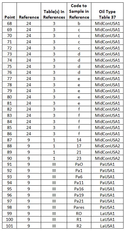
Experimental Data
Table 35
is the experimental data used by Hirschler to generate the ASTM D2502 chart.
The Chart Label column uses single characters for some figures to make them
more readable.


Table 36 contains tracking data for referencing back
to the original sources and the types of oils used to generate the data.


Calculation Codes
GW-BASIC
The code listing has inputs of the 2 viscosities and outputs
the calculated molecular weight.
There were some issues with using various forms of BASIC.
Some require line numbers and a termination line at the end of the listing;
others do not. In hexadecimal, the line termination line was 1A 20 0D 0A and in
decimal 26 32 13 10. These represent ASCII characters for SUB SPACE CR LF
(substitute[28], space, carriage return, line
feed). CR and LF are commonly used to terminal ASCII text files.
GW-BASIC Code listing:
10
Rem for V1 and V2 of 145 and 10
20
Rem the MWC is 398.3604
30
DEFINT K
40
DIM C(32)
50
C(1) = 4.11
60
C(2) = 1.358
70
C(3) = 1.5414
80
C(4) = -0.4106
90
C(5) = 197.6
100
C(6) = -592.944
110
C(7) = -96.08
120
C(8) = 0.8759
130
C(9) = 154.29
140
C(10) = -1.513
150
C(11) = 4.126
160
C(12) = 2.356
170
C(13) = 1.07
180
C(14) = 1.446
190
C(15) = -31.5
200
C(16) = -0.64
210
C(17) = 0.069
220
C(18) = 0.31
230
C(19) = -0.032
240
C(20) = 0.002
250
C(21) = -1.267
260
C(22) = 8.05
270
C(23) = -4.326
280
C(24) = 6.223
290
C(25) = 300
300
C(26) = -0.00326
310
C(27) = 19.54
320
C(28) = -30.387
330
C(29) = -12.02
340
C(30) = 7.276
350
C(31) = 6.498
360
C(32) = 52.3
370
INPUT "Enter Viscosity at 100F in cSt: ",V1
380
INPUT "Enter Viscosity at 210F in cSt: ",V2
390
F1=LOG(LOG(V1+C(1)))
400
F2=LOG(LOG(V2+C(2)))
410
F12=LOG(F1-C(3)*F2-C(4))
420
MW0=C(5)+C(6)*F12+C(7)*F12*F2^2+C(8)*F1^4+C(9)*F1*F2*F12
430
MWS=MW0*.01
440
FOR K=0 TO 1
450
K11=K*11
460
SI=SIN(C(10+K11))
470
CO=COS(C(10+K11))
480
X=(MWS*CO+F2*SI-C(11+K11)*CO-C(12+K11)*SI)/C(13+K11)
490
X2=X*X
500
Y=(F2*CO-C(12+K11)*CO-MWS*SI+C(11+K11)*SI)/C(14+K11)
510
Y2=Y*Y
520
EL=X2+Y2
530
SG=TAN(C(10+K11))*(-C(11+K11)+MWS)+C(12+K11)-F2
540
IF SC<0 THEN SG=-1 ELSE SG=1
550
EX=SG*EL
560
EX1=EX*(C(19+K11)+EX*C(20+K11))
570
EX2=EX*(C(17+K11)+EX*(C(18+K11)+EX1))
580
MW2=C(15+K11)*EXP(-(C(16+K11)+EX2))
590
IF K=0 THEN MW1=MW2
600
NEXT K
610
MWC=MW0+MW1+MW2+C(32)
620
PRINT USING "MWC= ####.####"; MWC
Excel VBA Functions
Molecular Weight Calculation Functions
There are 4 functions used to calculate the molecular weight
from viscosities at temperatures more common today than when the chart was
developed. The code for the functions is at the end
of this section.
1. MW40_100
is the top level function. Viscosities in cSt at 40°C, 100°C and the type of
viscosity
boundary error checking are the inputs. The function is hard coded to convert
viscosities from 40°C and 100°C to 37.778°C and 98.889°C (100°F and 210°F). It uses
the viscosity-temperature conversion function VisAtTC (Viscosity at Temperature
C)
and passes the converted viscosities to the MW function.
2.
VisAtTC converts the viscosities from two
temperatures to the viscosity at a 3rd
temperature. It is usable as
a standalone function as long as the required Log10 function
in VBA is
available.
3.
The Log10 function converts the native
VBA Log (base e) function to base 10[29]. As
a
standalone function, it is usable as needed in VBA. It is not for use in
spreadsheet cells as
the spreadsheet has both the Log and Ln as native
functions.
4.
The MW function calculates the molecular
weight using viscosities at 100°F and 210°F,
checks the viscosities for chart boundary
violations and returns the MW or boundary
violation code. It is usable as a
standalone function if V100 and V210 are the inputs.
MW Calculation from Viscosities at 40°C and 100°C
The function is MW40_100(V40C,V100C, optional Error Report
Code).
The molecular weight data used to check the viscosity
boundary violations was used to check the conversion of the viscosities from
100°F and 210°F to 40°C and 100°C and their use in this function. For all
values that are on the chart, the difference between the originally calculated
MWC and that from the viscosity converted MW40_100 version had a difference of <0.15.
Any values that showed larger differences had viscosities that would not be on
the chart, a V210 that was difficult to interpolate below 2.6 cSt (lower left
corner highlighted in yellow) or above 60 cSt. All the viscosity boundary
violations had the same error code except the point in the lower left corner of
the chart.
Table 38 Viscosities Converted to 40°C
and 100°C, Checked Against Previous Calculations


Conversion of Viscosity from 40°C and 100°C to 100°F and 210°F
The function is VisAtTC(p1, p2, p3, p4, p5). The parameter p1
represents the viscosity in cSt at the lower temperature p2 in Celsius. Parameters
p3 is the viscosity at the higher temperature p4. The parameter p5 is the
temperature in Celsius at which the viscosity is wanted.
The viscosity conversion uses the Wright equation[30],
which is the basis[31]
for ASTM D341[32].
Four sets of data were used to check VisAtTC (Viscosity at
Temperature C) function code against online calculations and gave comparable
results. Five other data sets were used to check its viscosity range (Table 39).
The differences seen on the low viscosities are irrelevant as they would not be
on the ASTM chart.
Table 39 Preliminary Testing of
Viscosity-Temperature Conversion Code

This function requires the use of the log (base 10) function,
which is not native to VBA. Included in the code list is the function Log10,
which converts the VBA natural Log (base e)
to the log base 10.
MW Calculation from Viscosities at 100°F and 210°F with Boundary Violation Discussion
The code is a VBA function MW(number1, number2, optional
text) that calculates the molecular weight using the method described in this
paper. It includes validating that both viscosities are within the chart area. The
inputs number1 and number2 are numbers or cell references to the viscosities
with number1 as the viscosity in cSt at 100°F and number2 as the viscosity in
cSt at 210°F. The optional text is either a text string in quotes or a cell
reference to text content. The optional text controls the type of error message
reported by the function.
The output is the calculated molecular weight or an error
code. The error codes will help determine which viscosities or which chart
boundaries are violated. The code terminology relates to the ASTM chart, as
that is more familiar than the modified charts (Figure 51
and Figure 52)
based on viscosity axes.

Boundary Violation Details
The ASTM D2502 chart has a distinct form (Figure 50).
Figure 50
shows the vertex points and boundary lines. The legend refers to those
boundaries on the chart. Table 42
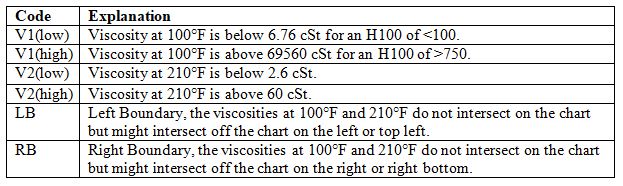
has the color-coding for the boundaries with descriptions and limits.
Table 42 Boundary Descriptions

The chart area below a V210 of 2.6 was not considered for
determining boundary limits because of the difficulty in determining the V210
at the point MW=220 and H100=100. The MWC estimates a viscosity of 1.927 cSt,
while estimating the point from the chart was between 1.725 (linear) and 1.95
(non-linear). Using the MWC value to fit the left boundary limit equation gave
a very high residual. If the higher residual for the corner point is used, the left
boundary constraint equation values would not flag V210 values that are well
off the chart and would be ineffective as a warning for invalid V210s.
A modified version of the chart (Figure 51)
used the viscosities for the axes. The legend and color-coding of the boundary
lines is consistent between the 2 charts. Some of the bottom boundaries are
difficult to discern and are visually clearer in Figure 52,
which is the same as Figure 51
but with both scales logarithmic. This helps with deciding how to set up the
boundary conditions.
Figure 50 Vertices and Boundary Lines on the
ASTM D2502 Chart

Figure 51 Fitting Data and Boundary Lines with
Viscosities as Axis


Equations were determined for both the right and left edges
(boundaries) of the ASTM chart. Table Curve 2D[35] fitted
V2 as a function of V1. The criterion for the function was the smallest standard
error that was consistent with a function that was rational, smoothly
increasing over the V1 range and computational straightforward to implement.
Consideration was not given to whether single or double precision was required.
There is no data for the left boundary of the chart from
previous work. An expanded digital picture was used to estimate the values for
the fit. Table 43
has the raw data values read or estimated from the ASTM chart, the input and
output for TC2D and a comparison of the chart MW with the MWC. The MWC compares
favorably to the chart MW with a standard deviation of 2.4 for the
difference between the chart MW and MWC. This is consistent with the standard
deviation for the chart fit in Table 4.
Table 43 Chart Points for Fitting Left Edge
Boundary Equation TC2D

Figure 52
is the left boundary calculation for V2 in terms of V1 from Table Curve 2D. The
function begins to become bimodal after the maximum V1. In Excel, the VBA MW
calculation function will never check for a V1> than the maximum for the
boundary, so the second value for V2 will not be encountered and cause the V2
value to be misreported as being on the chart when it is not.

Figure 53 Table Curve 2D Equation
Fitted to Left Edge of Chart
The boundary limit function and coefficients for the left
boundary are in Table 44.
The coefficients were initially single precision but it introduced some minor
differences in the calculated boundary values. Using double precision
eliminated the differences.
Table 44 Equation and Coefficient for Left
Boundary Limit of V210

The residuals in the calculated V210 were similar in scale
so an absolute value was used to adjust the boundary limit calculation. The
boundary limit calculated was adjusted by adding a value (-0.040) slightly less
than the largest negative fit residual for the data (-0.036 Table 43
point 21) and testing if V210 was < the adjusted limit. This assures that
none of the chart limit points would be incorrectly reported as out of bounds
due to residual fit errors. Figure 54
is a stylized graph with example values showing the methodology. At first
glance, the stylized graph may seem peculiar but it has to be referenced back to
Figure 51
with viscosity data, where the lower V100 boundary represents the left ASTM
chart boundary and the V210 data above the green line is V210 values on the
ASTM chart.
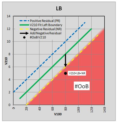
Figure 54 Stylized Chart Showing Adjustment to
the Left Boundary Limit
A similar procedure was done for the RB. The data is in Table 45.
There was some previous data on the RB and this was augmented with additional
points highlighted in yellow.


Figure 55 Table Curve 2D Equation
Fitted to Right Edge of Chart
The boundary limit function and coefficients for the right
boundary are in Table 46.

For the right boundary limit the methodology was similar but
the maximum residual was added and the test for OoB was V210 > the adjusted
limit. Again, the fit residuals were similar in scale so an absolute value was
used. The adjustment value added was slightly greater (0.110) than the largest positive
fit residual for the data (0.107 Table 46
point 9). This assures none of the chart boundary limit points would be
incorrectly reported as out of bounds due to residual fit errors. Figure 56
is a stylized graph with example values showing the methodology.

Figure 56 Stylized Chart Showing Adjustment to
the Right Boundary Limit
Testing the calculation against the experimental data from
the references gave 16 out of bounds points for the 19 experimental points in
reference 12. This agreed with previous evaluations of the data from that
reference. One additional point of the 37 points in reference 18 was out of
bounds. The V210 was 2.2 cSt. The boundary was set at 2.6 because the
non-linearity in the V210 isostokes made estimating viscosities in this area
difficult. The lower left corner was estimated to be H100=100 and V210=1.98 but
in setting up the boundary values, this viscosity gave an extremely high
residual for the fit and it was elected to make the lower boundary 2.6.
The
augmented left and right boundary data could be added to the fit data if the
coefficients for the MW calculation model were to be refined. Figure 57 shows the data point locations and is Figure
1 with the augmented boundary points. Figure
58 shows the residuals and is Figure 9 with the augmented boundary points. The points with white circles are
those that have residual >±4.5. These charts do not have the 3 corners
of the chart (bottom left, top left, bottom right) as boundary points (Table 47). The V210 viscosities for these points were estimated using the MWC
calculation to give the MW expected so the residuals are artificial and exactly
0. The left boundary corners gave high residual when fit to the boundary equation
than the lower right corner so it more realistically models that corner but
still had a residual high enough that it was not included in the fit.
Table 47 Boundary Points Not Use


Figure 57 All Data Points from the ASTM D2502
Chart

Figure 58 Residual for All Chart Points from
ASTM D2502
VBA Code
Molecular Weight Calculation Using Viscosities at 40°C and
100°C
Option
Explicit
Function
MW40_100(V40 As Double, V100 As Double, Optional ReportErr As String) As
Variant
'Joseph A. Weaver, Jr. 08/19/20
'Calculates the molecular weight (MW) of a petroleum oil from 2 viscosities
'Joseph A. Weaver, Jr. 08/19/20
'Calculates the molecular weight (MW) of a petroleum oil from 2 viscosities
' modeling ASTM D2502 chart but uses 40C and
100C cSt viscosities
'Input is V40 is viscosity at 40C in cSt, V100 is viscosity at 100C in cSt
'Input is V40 is viscosity at 40C in cSt, V100 is viscosity at 100C in cSt
' and optional ReportErr parameter for
checking and reporting viscosity validity.
' Default: "ReportErr" is missing or "" then reports viscosities are
' "#OoB" Out of Bounds and not on the chart
' "V" or "v" verbose: The function will report violations codes
' related to ASTM D2502 chart.
' "NC", "nc", "Nc", or "nC": Function does not check viscosities and
' report a molecular weight if there are no Excel calculation errors.
' Excel calculation errors with return #VALUE.
'Boundary Violation Codes
' "V1(low)" Viscosity at 100F is below 6.76 cSt = H100 of 100
' "V1(high)" Viscosity at 100F is above than 69560 cSt = H100 of 750
' "V2(low)" Viscosity at 210F is below 1.93 cSt (estimated low left corner of the chart)
' "V2(high)" Viscosity at 210F is above 60 cSt
' "LB" left boundary, The viscosity at 100F and 210 do not intersect on the chart
' but might intersect outside the left boundary or top left.
' "RB" right boundary, The viscosity at 100F and 210 do not intersect on the chart
' but might intersect outside the right boundary or right bottom.
' It can report a combination of these.
'It uses the VisAtTC to convert the viscosities from 40C and 100C in cSt to
' the viscosities in cSt at 37.777...F and 98.888...F
'The converted viscosities are input along with the ReportErr into the
' MW (molecular weight) calculation developed from 1980 to April 1985
' to model ASTM D2502
‘
Dim V100F As Double, V210F As Double, TCof100F As Double, TCof210F As Double
TCof100F = (100 - 32) * 5 / 9
TCof210F = (210 - 32) * 5 / 9
V100F = VisAtTC(V40, V100, 40, 100, TCof100F)
V210F = VisAtTC(V40, V100, 40, 100, TCof210F)
MW40_100 = MW(V100F, V210F, ReportErr)
End
Function
Viscosity-Temperature Conversion Code
Function
VisAtTC(V1c As Double, V2c As Double, T1C As Double, T2C As Double, T3C As
Double) As Double
‘Viscosity
at Temperature C
'Joseph
A. Weaver, Jr. 8/19/20
'Based
on the Wortley Andrew Wright equation Journal of Materials, JMLSA (1969), vol.
4.11 pp. 1927
'Converts
a petroleum oil viscosity to a viscosity at another temperature
'Requires
the viscosity of the oil at 2 temperatures
'V1c
and V2c are the viscosity in cSt at temperatures in Celsius T1C and T2C
'T3C
is the temperature in Celsius of the converted viscosity
'It
REQUIRES the LOG10 function below to calculate the base 10 log
' as VBA does not have this as a native
function
‘
Dim
V(2) As Double, C(2) As Double, Co(6, 6) As Double
Dim
K0 As Double, K1 As Double, TK(3) As Double
Dim
A As Double, B As Double
Dim
I As Integer, J As Integer, K As Integer
K0 =
273.15
K1 =
0.7
V(1)
= V1c
V(2)
= V2c
TK(1)
= T1C + K0
TK(2)
= T2C + K0
TK(3)
= T3C + K0
Co(1,
1) = -1.14883
Co(1,
2) = -2.65868
Co(2,
1) = -0.0038138
Co(2,
2) = -12.5645
Co(3,
1) = 5.46491
Co(3,
2) = -37.6289
Co(4,
1) = 13.0458
Co(4,
2) = -74.6851
Co(5,
1) = 37.4619
Co(5,
2) = -192.643
Co(6,
1) = 80.4945
Co(6,
2) = -400.468
I =
1
For
J = 1 To 2
C(J) = 0
For K = 1 To 6
C(J) = (-1) ^ (K + 1) * (Exp(Co(K, I) +
Co(K, I + 1) * V(J))) + C(J)
Next K
V(J) = V(J) + 0.7 + C(J)
Next
J
A =
(Log10(Log10(V(2))) - Log10(Log10(V(1))) * Log10(TK(2)) / Log10(TK(1))) / (1 -
Log10(TK(2)) / Log10(TK(1)))
B =
(A - Log10(Log10(V(1)))) / Log10(TK(1))
VisAtTC
= 10 ^ (10 ^ (A - B * Log10(TK(3)))) - 0.7
End
Function
Conversion Code for Log to base e to Base 10
Function
Log10(Arg1 As Double) As Double
'Converts the VBA Log (base e) function to base 10 as
'VBA does not have a native Log base 10 function
Log10 = Log(Arg1) / Log(10#)
End Function
'Converts the VBA Log (base e) function to base 10 as
'VBA does not have a native Log base 10 function
Log10 = Log(Arg1) / Log(10#)
End Function
Molecular Weight Calculation Using Viscosities at 100°F and
210°F
Function
MW(V1 As Single, V2 As Single, Optional ReportErr As String) As Variant
'Joseph A. Weaver, Jr. 08/19/20
'Calculates the molecular weight (MW) of a petroleum oil from the 2 viscosities
' used to make the ASTM D2502 chart
'Input is V1 is viscosity at 100F in cSt, V2 is viscosity at 100F in cSt
' and optional ReportErr parameter for checking and reporting viscosity validity.
' Default: "ReportErr" is missing or "" then reports viscosities are
' "#OoB" Out of Bounds and not on the chart
' "V" or "v" verbose: The function will report violations codes
' related to ASTM D2502 chart.
' "NC", "nc", "Nc", or "nC": Function does not check viscosities and
' report a molecular weight if there are no Excel calculation errors.
' Excel calculation errors with return #VALUE.
'Boundary Violation Codes
' "V1(low)" Viscosity at 100F is below 6.76 cSt = H100 of 100
' "V1(high)" Viscosity at 100F is above than 69560 cSt = H100 of 750
' "V2(low)" Viscosity at 210F is below 1.93 cSt (estimated low left corner of the chart)
' "V2(high)" Viscosity at 210F is above 60 cSt
' "LB" left boundary, The viscosity at 100F and 210 do not intersect on the chart
' but might intersect outside the left boundary or top left.
' "RB" right boundary, The viscosity at 100F and 210 do not intersect on the chart
' but might intersect outside the right boundary or right bottom.
' It can report a combination of these.
'It uses the VisAtTC to convert the viscosities from 40C and 100C in cSt to
' the viscosities in cSt at 37.777...F and 98.888...F
'The converted viscosities are input along with the ReportErr into the
' MW (molecular weight) calculation developed from 1980 to April 1985
' to model ASTM D2502
'It has been augmented 08/15/20 to check that the viscosities will be
' in the range of the chart
‘
MW = ""
ReportErr = UCase(ReportErr)
'Initialize Viscosities Min Max and constrained
Dim V1Min As Single, V1MaxRB As Single, V1Max As Single
Dim V2Min As Single, V2MinRB As Single, V2Max As Single
Dim NumVisOutOfRange As Integer
V1Min = 6.7590916903038
V1MaxRB = 2247.7890693438
V1Max = 69560.1787709072
‘V2Min = 1.92659741640091
V2Min = 2.6
V2MinRB = 4.25037789344788
V2Max = 60
NumVisOutOfRange = 0
'Left Boundary Parameters and Calculation
'The calculation in VBA and the worksheet gave different result
'unless the LB coefficients were defined as double
Dim LB(11) As Double, LBVal As Single, LBTol As Single
LB(1) = 140012.095739587
LB(2) = -23114.7634370257
LB(3) = -572807.982232585
LB(4) = 2543.00575316951
LB(5) = 1564758.63486259
LB(6) = -178.300226912808
LB(7) = -2735170.67925539
LB(8) = 7.19443368988872
LB(9) = 2766419.62786965
LB(10) = -0.126905455696835
LB(11) = -1231167.60935815
'y=a+blnx+c/lnx+d(lnx)^2+e/(lnx)^2+f(lnx)^3+g/(lnx)^3+h(lnx)^4+i/(lnx)^4+j(lnx)^5+k/(lnx)^5
LBVal = LB(1) + LB(2) * Log(V1) + LB(3) / Log(V1) + LB(4) * Log(V1) ^ 2 _
+ LB(5) / Log(V1) ^ 2 + LB(6) * Log(V1) ^ 3 + LB(7) / Log(V1) ^ 3 _
+ LB(8) * Log(V1) ^ 4 + LB(9) / Log(V1) ^ 4 + LB(10) * Log(V1) ^ 5 _
+ LB(11) / Log(V1) ^ 5
'Maximum residual added to boundary calculation to make sure V2 <= boundary across all values
'Residual from fit -0.036 to 0.043
LBTol = -0.04
LBVal = LBVal + LBTol
'Right Boundary Parameters and Calculations
Dim RB(7) As Single, RBVal As Single, RBMinV2 As Single, RBTol As Single
RB(1) = 0.545817589635799
RB(2) = 1.44245021850922
RB(3) = -1.31564083827617E-02
RB(4) = 1.83490105482591E-03
RB(5) = -1.14182344081125E-04
RB(6) = 2.72843501043909E-06
RB(7) = -2.21517012538976E-08
'y=a+bx^(0.5)+cx+dx^(1.5)+ex^2+fx^(2.5)+gx^3
RBVal = RB(1) + RB(2) * V1 ^ 0.5 + RB(3) * V1 + RB(4) * V1 ^ 1.5 + RB(5) _
* V1 ^ 2 + RB(6) * V1 ^ 2.5 + RB(7) * V1 ^ 3
'Minimum residual added to boundary calculation to make sure V2 >= boundary
' across all values
'Residual from fit -0.172 to 0.107
RBTol = 0.11
RBVal = RBVal + RBTol
If
ReportErr = "NC" Then GoTo SkipInputCheck
'Check if V1 is too high or low
If V1 < V1Min Then
MW = "V1(low) "
NumVisOutOfRange = NumVisOutOfRange + 1
End If
If V1 > V1Max Then
MW = "V1(high) "
NumVisOutOfRange = NumVisOutOfRange + 1
End If
If V2 < V2Min Then
MW = MW + "V2(low) "
NumVisOutOfRange = NumVisOutOfRange + 1
End If
If V2 > V2Max Then
MW = MW + "V2(high) "
NumVisOutOfRange = NumVisOutOfRange + 1
End If
If NumVisOutOfRange = 2 Then GoTo SkipEdgeCheck
'Check
left boundary for valid V1&V2
If V1 >= V1Min And V1 <= V1Max Then
If V2 < LBVal Then MW = MW + "LB"
End If
'Check
Right boundary for valid V1&V2
If V1 >= V1Min And V1 <= V1MaxRB Then
If V2 > RBVal Then MW = MW + "RB"
End If
SkipEdgeCheck:
If MW <> "" And ReportErr = "V" Then
'Assures that only "V" input will report codes in MW
Else
If MW <> "" Then MW = "#OoB"
End If
' Debug.Print MW
If MW <> "" Then Exit Function
SkipInputCheck:
'Coefficients
Dim C(32) As Single
C(1) = 4.11
C(2) = 1.358
C(3) = 1.5414
C(4) = -0.4106
C(5) = 197.6
C(6) = -592.944
C(7) = -96.08
C(8) = 0.8759
C(9) = 154.29
C(10) = -1.513
C(11) = 4.126
C(12) = 2.356
C(13) = 1.07
C(14) = 1.446
C(15) = -31.5
C(16) = -0.64
C(17) = 0.069
C(18) = 0.31
C(19) = -0.032
C(20) = 0.002
C(21) = -1.267
C(22) = 8.05
C(23) = -4.326
C(24) = 6.223
C(25) = 300
C(26) = -0.00326
C(27) = 19.54
C(28) = -30.387
C(29) = -12.02
C(30) = 7.276
C(31) = 6.498
C(32) = 52.3
Dim
K As Integer, K11 As Integer
Dim F1 As Single, F2 As Single, F12 As Single
Dim MW0 As Single, MW1 As Single, MW2 As Single, MWS As Single, MWC As Single
Dim X As Single, X2 As Single, Y As Single, Y2 As Single, EL As Single
Dim SI As Single, CO As Single
Dim SG As Single, EX As Single, EX1 As Single, EX2 As Single
'MW Calculation
F1 = Log(Log(V1 + C(1)))
F2 = Log(Log(V2 + C(2)))
F12 = Log(F1 - C(3) * F2 - C(4))
MW0 = C(5) + C(6) * F12 + C(7) * F12 * F2 ^ 2 + C(8) * F1 ^ 4 + C(9) * F1 * F2 * F12
MWS = MW0 * 0.01
For K = 0 To 1
K11 = K * 11
SI = Sin(C(10 + K11))
CO = Cos(C(10 + K11))
X = (MWS * CO + F2 * SI - C(11 + K11) * CO - C(12 + K11) * SI) / C(13 + K11)
X2 = X * X
Y = (F2 * CO - C(12 + K11) * CO - MWS * SI + C(11 + K11) * SI) / C(14 + K11)
Y2 = Y * Y
EL = X2 + Y2
SG = Tan(C(10 + K11)) * (-C(11 + K11) + MWS) + C(12 + K11) - F2
If SG < 0 Then SG = -1 Else SG = 1
EX = SG * EL
EX1 = EX * (C(19 + K11) + EX * C(20 + K11))
EX2 = EX * (C(17 + K11) + EX * (C(18 + K11) + EX1))
MW2 = C(15 + K11) * Exp(-(C(16 + K11) + EX2))
If K = 0 Then MW1 = MW2
Next
MWC = MW0 + MW1 + MW2 + C(32)
MW = MWC
'Joseph A. Weaver, Jr. 08/19/20
'Calculates the molecular weight (MW) of a petroleum oil from the 2 viscosities
' used to make the ASTM D2502 chart
'Input is V1 is viscosity at 100F in cSt, V2 is viscosity at 100F in cSt
' and optional ReportErr parameter for checking and reporting viscosity validity.
' Default: "ReportErr" is missing or "" then reports viscosities are
' "#OoB" Out of Bounds and not on the chart
' "V" or "v" verbose: The function will report violations codes
' related to ASTM D2502 chart.
' "NC", "nc", "Nc", or "nC": Function does not check viscosities and
' report a molecular weight if there are no Excel calculation errors.
' Excel calculation errors with return #VALUE.
'Boundary Violation Codes
' "V1(low)" Viscosity at 100F is below 6.76 cSt = H100 of 100
' "V1(high)" Viscosity at 100F is above than 69560 cSt = H100 of 750
' "V2(low)" Viscosity at 210F is below 1.93 cSt (estimated low left corner of the chart)
' "V2(high)" Viscosity at 210F is above 60 cSt
' "LB" left boundary, The viscosity at 100F and 210 do not intersect on the chart
' but might intersect outside the left boundary or top left.
' "RB" right boundary, The viscosity at 100F and 210 do not intersect on the chart
' but might intersect outside the right boundary or right bottom.
' It can report a combination of these.
'It uses the VisAtTC to convert the viscosities from 40C and 100C in cSt to
' the viscosities in cSt at 37.777...F and 98.888...F
'The converted viscosities are input along with the ReportErr into the
' MW (molecular weight) calculation developed from 1980 to April 1985
' to model ASTM D2502
'It has been augmented 08/15/20 to check that the viscosities will be
' in the range of the chart
‘
MW = ""
ReportErr = UCase(ReportErr)
'Initialize Viscosities Min Max and constrained
Dim V1Min As Single, V1MaxRB As Single, V1Max As Single
Dim V2Min As Single, V2MinRB As Single, V2Max As Single
Dim NumVisOutOfRange As Integer
V1Min = 6.7590916903038
V1MaxRB = 2247.7890693438
V1Max = 69560.1787709072
‘V2Min = 1.92659741640091
V2Min = 2.6
V2MinRB = 4.25037789344788
V2Max = 60
NumVisOutOfRange = 0
'Left Boundary Parameters and Calculation
'The calculation in VBA and the worksheet gave different result
'unless the LB coefficients were defined as double
Dim LB(11) As Double, LBVal As Single, LBTol As Single
LB(1) = 140012.095739587
LB(2) = -23114.7634370257
LB(3) = -572807.982232585
LB(4) = 2543.00575316951
LB(5) = 1564758.63486259
LB(6) = -178.300226912808
LB(7) = -2735170.67925539
LB(8) = 7.19443368988872
LB(9) = 2766419.62786965
LB(10) = -0.126905455696835
LB(11) = -1231167.60935815
'y=a+blnx+c/lnx+d(lnx)^2+e/(lnx)^2+f(lnx)^3+g/(lnx)^3+h(lnx)^4+i/(lnx)^4+j(lnx)^5+k/(lnx)^5
LBVal = LB(1) + LB(2) * Log(V1) + LB(3) / Log(V1) + LB(4) * Log(V1) ^ 2 _
+ LB(5) / Log(V1) ^ 2 + LB(6) * Log(V1) ^ 3 + LB(7) / Log(V1) ^ 3 _
+ LB(8) * Log(V1) ^ 4 + LB(9) / Log(V1) ^ 4 + LB(10) * Log(V1) ^ 5 _
+ LB(11) / Log(V1) ^ 5
'Maximum residual added to boundary calculation to make sure V2 <= boundary across all values
'Residual from fit -0.036 to 0.043
LBTol = -0.04
LBVal = LBVal + LBTol
'Right Boundary Parameters and Calculations
Dim RB(7) As Single, RBVal As Single, RBMinV2 As Single, RBTol As Single
RB(1) = 0.545817589635799
RB(2) = 1.44245021850922
RB(3) = -1.31564083827617E-02
RB(4) = 1.83490105482591E-03
RB(5) = -1.14182344081125E-04
RB(6) = 2.72843501043909E-06
RB(7) = -2.21517012538976E-08
'y=a+bx^(0.5)+cx+dx^(1.5)+ex^2+fx^(2.5)+gx^3
RBVal = RB(1) + RB(2) * V1 ^ 0.5 + RB(3) * V1 + RB(4) * V1 ^ 1.5 + RB(5) _
* V1 ^ 2 + RB(6) * V1 ^ 2.5 + RB(7) * V1 ^ 3
'Minimum residual added to boundary calculation to make sure V2 >= boundary
' across all values
'Residual from fit -0.172 to 0.107
RBTol = 0.11
RBVal = RBVal + RBTol
'Check if V1 is too high or low
If V1 < V1Min Then
MW = "V1(low) "
NumVisOutOfRange = NumVisOutOfRange + 1
End If
If V1 > V1Max Then
MW = "V1(high) "
NumVisOutOfRange = NumVisOutOfRange + 1
End If
If V2 < V2Min Then
MW = MW + "V2(low) "
NumVisOutOfRange = NumVisOutOfRange + 1
End If
If V2 > V2Max Then
MW = MW + "V2(high) "
NumVisOutOfRange = NumVisOutOfRange + 1
End If
If NumVisOutOfRange = 2 Then GoTo SkipEdgeCheck
If V1 >= V1Min And V1 <= V1Max Then
If V2 < LBVal Then MW = MW + "LB"
End If
If V1 >= V1Min And V1 <= V1MaxRB Then
If V2 > RBVal Then MW = MW + "RB"
End If
SkipEdgeCheck:
If MW <> "" And ReportErr = "V" Then
'Assures that only "V" input will report codes in MW
Else
If MW <> "" Then MW = "#OoB"
End If
' Debug.Print MW
If MW <> "" Then Exit Function
SkipInputCheck:
Dim C(32) As Single
C(1) = 4.11
C(2) = 1.358
C(3) = 1.5414
C(4) = -0.4106
C(5) = 197.6
C(6) = -592.944
C(7) = -96.08
C(8) = 0.8759
C(9) = 154.29
C(10) = -1.513
C(11) = 4.126
C(12) = 2.356
C(13) = 1.07
C(14) = 1.446
C(15) = -31.5
C(16) = -0.64
C(17) = 0.069
C(18) = 0.31
C(19) = -0.032
C(20) = 0.002
C(21) = -1.267
C(22) = 8.05
C(23) = -4.326
C(24) = 6.223
C(25) = 300
C(26) = -0.00326
C(27) = 19.54
C(28) = -30.387
C(29) = -12.02
C(30) = 7.276
C(31) = 6.498
C(32) = 52.3
Dim F1 As Single, F2 As Single, F12 As Single
Dim MW0 As Single, MW1 As Single, MW2 As Single, MWS As Single, MWC As Single
Dim X As Single, X2 As Single, Y As Single, Y2 As Single, EL As Single
Dim SI As Single, CO As Single
Dim SG As Single, EX As Single, EX1 As Single, EX2 As Single
F1 = Log(Log(V1 + C(1)))
F2 = Log(Log(V2 + C(2)))
F12 = Log(F1 - C(3) * F2 - C(4))
MW0 = C(5) + C(6) * F12 + C(7) * F12 * F2 ^ 2 + C(8) * F1 ^ 4 + C(9) * F1 * F2 * F12
MWS = MW0 * 0.01
For K = 0 To 1
K11 = K * 11
SI = Sin(C(10 + K11))
CO = Cos(C(10 + K11))
X = (MWS * CO + F2 * SI - C(11 + K11) * CO - C(12 + K11) * SI) / C(13 + K11)
X2 = X * X
Y = (F2 * CO - C(12 + K11) * CO - MWS * SI + C(11 + K11) * SI) / C(14 + K11)
Y2 = Y * Y
EL = X2 + Y2
SG = Tan(C(10 + K11)) * (-C(11 + K11) + MWS) + C(12 + K11) - F2
If SG < 0 Then SG = -1 Else SG = 1
EX = SG * EL
EX1 = EX * (C(19 + K11) + EX * C(20 + K11))
EX2 = EX * (C(17 + K11) + EX * (C(18 + K11) + EX1))
MW2 = C(15 + K11) * Exp(-(C(16 + K11) + EX2))
If K = 0 Then MW1 = MW2
Next
MWC = MW0 + MW1 + MW2 + C(32)
MW = MWC
End
Function
Conversion of SUS and cSt, VBA Code and Cell Formula:
It is difficult to algebraically manipulate the ASTM
calculation to convert cSt to SUS in equation {1} to give a reverse calculation
(InvSUS).
An-in cell calculation was developed that used a reiterative
calculation with successive approximations. This became the basis for a VBA function.
The VBA code for conversion of cSt to SUS is;
Function
cSt40From(SUSAt100 As Single, Optional Temp As Single = 104) As Single
'Calculates SUS from cSt at 40C (104F) based on ASTM D 2161
'Temp is the temperature of the cSt in F (40C =104F exactly)other cSt temperatures can be used
'The calculation from cSt to SUS is done iteratively and takes about 6 loops.
‘Joseph A. Weaver, Jr. 2010
'Calculates SUS from cSt at 40C (104F) based on ASTM D 2161
'Temp is the temperature of the cSt in F (40C =104F exactly)other cSt temperatures can be used
'The calculation from cSt to SUS is done iteratively and takes about 6 loops.
‘Joseph A. Weaver, Jr. 2010
Dim
SUS1 As Double
Dim SUS2 As Double
Dim SUSd As Double
Dim cSt1 As Double
SUS1 = SUSAt100
cSt1 = SUS1 / 4.6324
SUS2 = (1 + 0.000061 * (Temp - 100)) * (4.6324 * cSt1 + (1 + 0.03264 * cSt1) / ((3930.2 + 262.7 * cSt1 + 23.97 * cSt1 ^ 2 + 1.646 * cSt1 ^ 3) * 0.00001))
SUSd = SUS1 - SUS2
Dim SUS2 As Double
Dim SUSd As Double
Dim cSt1 As Double
SUS1 = SUSAt100
cSt1 = SUS1 / 4.6324
SUS2 = (1 + 0.000061 * (Temp - 100)) * (4.6324 * cSt1 + (1 + 0.03264 * cSt1) / ((3930.2 + 262.7 * cSt1 + 23.97 * cSt1 ^ 2 + 1.646 * cSt1 ^ 3) * 0.00001))
SUSd = SUS1 - SUS2
Do
Until Abs(SUSd) < 0.000001
cSt1 = cSt1 + SUSd / 4.6324
SUS2 = (1 + 0.000061 * (Temp - 100)) *
(4.6324 * cSt1 + (1 + 0.03264 * cSt1) / ((3930.2 + 262.7 * cSt1 + 23.97 * cSt1
^ 2 + 1.646 * cSt1 ^ 3) * 0.00001))
SUSd = SUSAt100 - SUS2
SUS1 = SUSAt100 + SUSd
Loop
cSt40From
= cSt1
End
Function
The circular 1-cell calculation based on the iteration
calculation feature of Excel refines the cSt (InvSUS) by successively reducing
the difference between a calculated SUS value and the SUS entered for
conversion. Further below is the procedure to
set up Excel and use the calculation.
The InvSUS calculation used reiteratively in Excel is
cSt =
A2+B2- {2}
(1+0.000061*(C2-100))* {3}
(4.6324*A2+(1+0.03264*A2)/((3930.2+262.7*A2+23.97*A2^2+1.646*A2^3)*0.00001)) {4}
)*0.1 {5}
where
Excel
cell Content
A2 contains the formula {6}
InvSUS to calculate SUS from cSt
B2 SUS viscosity
C2 temperature °F
Lines {3} and {4}, which uses the ASTM D2161 calculation for
converting cSt to SUS, calculates an new estimate of temperature corrected SUS
from the cSt previously calculated in A2 (circular self referencing). The newly
estimated SUS ({3} and {4}) is subtracted from the SUS being converted (B2 in
line {2}) to give the error. Ten percent (0.1, line {5}) of the error is added
to the value previously in A2 and Excel places the new value in A2. This is
repeated until the limit of the Maximum Iterations or the Maximum Change
options iterations is reached. Typically, it takes about 23 iterations to reach
a precision of 0.001. For a precision of 0.0000000000001, it takes about 75
iterations. Calculating SUS to a cSt and that value back to SUS showed no
difference between the initial SUS and final SUS.
For copy and pasting into
Excel the one line version of InvSUS (cSt) is
= A2+(B2-(1+0.000061*(C2-100))*(4.6324*A2+(1+0.03264*A2)/((3930.2+262.7*A2+23.97*A2^2+1.646*A2^3)*0.00001)))*0.1 {6}
To use {6} the calculation options must have iterative calculation
enabled. Any changes will affect all open workbooks[36].
To access and set up the
iterative calculation in Excel 2007:
1.
click on the Application
button ,
,
 ,
,2. select Excel Options at the bottom,
3. select Formulas on the left side bar,
4. in the Calculation Options panel on the right click on
the Automatic circular radio button,
5. click on Enable iterative calculation box to check it,
6. set Maximum Iterations: box to 100
7. set the Maximum Change: box to 0.001
8. click on the OK button at the bottom.
To use equation {6}:
1.
copy
and paste the green highlighted of {6} into cell A2
Calculation {6} is on two lines but
has no return or paragraph mark so it pastes as a
formula in the cell.
If the iterative calculation is not
enabled, a “Circular Reference Warning” will appear and
the iterative
calculation will have to be enabled. The iterative calculation may or may not
be permanently stored with the workbook[37].
2. enter
the SUS to be converted into cell B2,
3. enter
the °F temperature in C2 , which is usually 100 or 210.
4. cell
A2 will have the result.
5. If
equation {6} is used in other cells, it will have to be edited to refer to them
For completeness, the VBA calculation function to convert
cSt to SUS is:
Function
SUS100From(cStAtTemp As Single, Optional Temp As Single = 104) As Single
'Calculates SUS at 100F from cSt at 40C based on ASTM D 2161
'Temp is the temperature of the cSt in F (40C =104F exactly) - other cSt temperatures can be used
SUS100From = (1 + 0.000061 * (Temp - 100)) * (4.6324 * cStAtTemp + (1 + 0.03264 * cStAtTemp) / ((3930.2 + 262.7 * cStAtTemp + 23.97 * cStAtTemp ^ 2 + 1.646 * cStAtTemp ^ 3) * 0.00001))
End Function
Chebyshev Bivariate 10th Order Polynomial C++ Code
NOTE: The x and y
input is H100 and H210 NOT V100 and V210 so the viscosities would have to be preprocessed to use the code.
There is no check if H100 or H210
are in the valid range of the ASTM D2502 chart.
In C++ log is to the base e.
The C++ code was not edited to show it as Log.
C++ Code listing:
/*--------------------------------------------------------------*
TableCurve 3D CPP Code Output
To modify generated output, edit CPP.TCL
Joseph
A. Weaver, Jr. 07/18/2020 Notes added
CPP is C++, NOTE x and y are the H100 and H210 functions
calculated from the viscosity at 100F in cSt (V100) and
210F (V210) using the calculations H100=870*Log(Log(V100
+ 0.6))+154 and H210=870*Log(Log(V210 + 0.6))+154
*--------------------------------------------------------------*/
#include
<math.h>
#include <stdio.h>
class
eqn409
{
public:
eqn409(){ XLo=104.3; XHi=750; YLo=-104.0243053; YHi=372.3898956; }
~eqn409(){}
double Eval(double x, double y);
int RootsX(double y, double z, double *roots, int maxcnt=10, double xlo=0.0, double xhi=0.0);
int RootsY(double x, double z, double *roots, int maxcnt=10, double ylo=0.0, double yhi=0.0);
protected:
int Roots(double fixed, double z, double *roots, int maxcnt, double varlo, double varhi, int isvarx);
private:
double XLo,XHi,YLo,YHi;
};
void
main(void)
{
int i,ix,iy;
double x,y,z,xr[10],yr[10];
char str[80];
eqn409 *e = new eqn409();
while(1){
printf("Enter x: ");
gets(str);
if(!*str) break;
sscanf(str,"%lg",&x);
printf("Enter y: ");
gets(str);
if(!*str) break;
sscanf(str,"%lg",&y);
z = e->Eval(x,y);
ix = e->RootsX(y,z,xr);
iy = e->RootsY(x,z,yr);
printf(" z=%.15lg\n",z);
for(i=0; i<ix; i++)
printf(" x root at [y,z]=%.15lg\n",xr[i]);
for(i=0; i<iy; i++)
printf(" y root at [x,z]=%.15lg\n",yr[i]);
}
delete e;
}
class
CEvalChebPoly
{
public:
CEvalChebPoly(int Order, int LogX, int LogY, double *Parms, double Scale0, double Scale1,
double Scale2, double Scale3, double Scale4, double Scale5, double Scale6, double Scale7){
order=Order; logx=LogX; logy=LogY; p=Parms;
s0=Scale0; s1=Scale1; s2=Scale2; s3=Scale3; s4=Scale4; s5=Scale5; s6=Scale6; s7=Scale7;
}
~CEvalChebPoly(){}
double Eval(double x, double y);
private:
int order, logx, logy;
double *p, s0, s1, s2, s3, s4, s5, s6, s7;
};
double CEvalChebPoly::Eval(double x, double y)
{
int tcnt,j,m,iv;
double tx[12],ty[12],v[70],ans;
if(!logx) x=(x-s0)/s1;
else x=(log(x)-s2)/s3;
if(!logy) y=(y-s4)/s5;
else y=(log(y)-s6)/s7;
switch(order){
case 5: tcnt=3; break;
case 9: tcnt=4; break;
case 14: tcnt=5; break;
case 20: tcnt=6; break;
case 27: tcnt=7; break;
case 35: tcnt=8; break;
case 44: tcnt=9; break;
case 54: tcnt=10; break;
case 65: tcnt=11; break;
default: return 0.0;
}
if(tcnt>6){
if(x<-1.0) x=-1.0;
if(x>1.0) x= 1.0;
if(y<-1.0) y=-1.0;
if(y>1.0) y= 1.0;
}
tx[0]=ty[0]=1.0;
tx[1]=x; ty[1]=y;
for(j=2;j<tcnt;j++){
tx[j]=2*x*tx[j-1]-tx[j-2];
ty[j]=2*y*ty[j-1]-ty[j-2];
}
iv=0;
for(j=0;j<tcnt;j++){
for(m=j; m>=0; m--)
v[iv++]=tx[m]*ty[j-m];
}
ans=0.0;
for(j=0;j<=order;j++)
ans += p[j]*v[j];
return ans;
}
double
eqn409::Eval(double x, double y)
/*--------------------------------------------------------------*
TableCurve 3D
File Source= z:\hhmwfit.txt
Date= Jul 18, 2020
Time= 0:14:49 AM
Data Set= hhmwfit.txt, X , Y , Z
X=
Y=
Z=
Eqn#= 409
Eqn= Chebyshev X,Y Bivariate Polynomial Order 10
r2=0.999913899675761
r2adj=0.9998540826083949
StdErr=1.735624555169359
Fstat=17152.03660867905
a= 68764722.53589136
b= 28756470.71514429
c= -28979595.67667712
d= 95177034.75920626
e= -229982373.5206862
f= 97092667.93893693
g= 12569683.13775275
h= -38351570.13231931
i= 39252125.19130948
j= -13476720.83923102
k= 30709893.98453927
l= -108737098.5923456
m= 132747209.3528934
n= -113137642.8373347
o= 33227767.91511252
p= 2210622.296494415
q= -10660333.93822856
r= 16572348.0760467
s= -17227243.48209736
t= 11974585.28015124
u= -2683099.775541091
v= 4218182.280174093
aa= -22905905.57409191
ab= 41034779.01510019
ac= -50626098.48131823
ad= 43529710.5471436
ae= -25742538.44318724
af= 5008018.216648622
ag= 126060.7178656597
ah= -1072545.105023687
ai= 2653713.014563096
aj= -4211585.987928544
ak= 4446945.663222158
al= -3123361.193343093
am= 1406400.919557086
an= -184036.4261667721
ao= 201554.839972609
ap= -1854263.583254318
aq= 5096769.362522405
ar= -9240567.062948906
as= 11520713.29494397
at= -9987286.810286814
au= 5937407.288753645
av= -2314246.129918459
ba= 266729.2466010882
bb= 1297.672695887418
bc= -26214.83213007698
bd= 115893.3501681627
be= -295493.5573140769
bf= 479746.6641668526
bg= -514563.3816430145
bh= 364433.9830717448
bi= -164155.3575705012
bj= 42597.36066984419
bk= -2420.107626222836
bl= 1973.035134363025
bm= -39945.61001880958
bn= 185159.4332253456
bo= -514410.5164602132
bp= 943363.2102345941
bq= -1188169.123533947
br= 1037703.359409076
bs= -619120.0327639152
bt= 241003.9999587515
bu= -55146.10647030385
bv= 2808.54446405081
*--------------------------------------------------------------*/
{
double z;
static double c[]= {
68764722.53589136,
28756470.71514429,
-28979595.67667712,
95177034.75920626,
-229982373.5206862,
97092667.93893693,
12569683.13775275,
-38351570.13231931,
39252125.19130948,
-13476720.83923102,
30709893.98453927,
-108737098.5923456,
132747209.3528934,
-113137642.8373347,
33227767.91511252,
2210622.296494415,
-10660333.93822856,
16572348.07604670,
-17227243.48209736,
11974585.28015124,
-2683099.775541091,
4218182.280174093,
-22905905.57409191,
41034779.01510019,
-50626098.48131823,
43529710.54714360,
-25742538.44318724,
5008018.216648622,
126060.7178656597,
-1072545.105023687,
2653713.014563096,
-4211585.987928544,
4446945.663222158,
-3123361.193343093,
1406400.919557086,
-184036.4261667721,
201554.8399726090,
-1854263.583254318,
5096769.362522405,
-9240567.062948906,
11520713.29494397,
-9987286.810286814,
5937407.288753645,
-2314246.129918459,
266729.2466010882,
1297.672695887418,
-26214.83213007698,
115893.3501681627,
-295493.5573140769,
479746.6641668526,
-514563.3816430145,
364433.9830717448,
-164155.3575705012,
42597.36066984419,
-2420.107626222836,
1973.035134363025,
-39945.61001880958,
185159.4332253456,
-514410.5164602132,
943363.2102345941,
-1188169.123533947,
1037703.359409076,
-619120.0327639152,
241003.9999587515,
-55146.10647030385,
2808.544464050810,
};
CEvalChebPoly *e = new CEvalChebPoly(65,0,0,c,
427.1500000000000,322.8500000000000,
5.633672284268541,0.9864009222618147,
134.1827951500000,238.2071004500000,
0.000000000000000,0.000000000000000);
z = e->Eval(x,y);
delete e;
return z;
}
int eqn409::Roots(double fixed, double z, double *roots, int maxcnt, double varlo, double varhi, int isvarx)
{
int i,j,k=0;
double v1,v2,vl,vh,vctr,dv,f,fmid,vmid,rt,vacc,delta;
if(varlo==0.0 && varhi==0.0){
vl=(isvarx)? XLo : YLo;
vh=(isvarx)? XHi : YHi;
}
else{ vl=varlo; vh=varhi; }
delta=(vh-vl)*0.01;
for(i=0; i<100; i++){
v1=vl+((double)i+1e-8)*delta;
v2=vl+((double)(i+1)+1e-8)*delta;
vctr=(v1+v2)*0.5;
vacc=(vctr==0)?1e-8:fabs(1e-8*vctr);
f=z-((isvarx)? Eval(v1,fixed) : Eval(fixed,v1));
fmid=z-((isvarx)? Eval(v2,fixed) : Eval(fixed,v2));
if(f*fmid >=0.0)
continue;
if(f<0.0){
dv=v2-v1;
rt=v1;
}
else{
dv=v1-v2;
rt=v2;
}
for(j=1; j<=100; j++){
dv *= 0.5;
vmid=rt+dv;
fmid=z-((isvarx)? Eval(vmid,fixed) : Eval(fixed,vmid));
if(fmid<=0)
rt=vmid;
if(fabsl(dv)<vacc || fmid==0.0){
if(k<maxcnt)
roots[k++]=rt;
if(k==maxcnt) return k;
break;
}
}
}
return k;
}
int eqn409::RootsX(double y, double z, double *xr, int maxcnt, double xlo, double xhi)
{
return Roots(y,z,xr,maxcnt,xlo,xhi,1);
}
int eqn409::RootsY(double x, double z, double *yr, int maxcnt, double ylo, double yhi)
{
return Roots(x,z,yr,maxcnt,ylo,yhi,0);
}
TableCurve 3D CPP Code Output
To modify generated output, edit CPP.TCL
CPP is C++, NOTE x and y are the H100 and H210 functions
calculated from the viscosity at 100F in cSt (V100) and
210F (V210) using the calculations H100=870*Log(Log(V100
+ 0.6))+154 and H210=870*Log(Log(V210 + 0.6))+154
*--------------------------------------------------------------*/
#include <stdio.h>
{
public:
eqn409(){ XLo=104.3; XHi=750; YLo=-104.0243053; YHi=372.3898956; }
~eqn409(){}
double Eval(double x, double y);
int RootsX(double y, double z, double *roots, int maxcnt=10, double xlo=0.0, double xhi=0.0);
int RootsY(double x, double z, double *roots, int maxcnt=10, double ylo=0.0, double yhi=0.0);
protected:
int Roots(double fixed, double z, double *roots, int maxcnt, double varlo, double varhi, int isvarx);
private:
double XLo,XHi,YLo,YHi;
};
{
int i,ix,iy;
double x,y,z,xr[10],yr[10];
char str[80];
eqn409 *e = new eqn409();
while(1){
printf("Enter x: ");
gets(str);
if(!*str) break;
sscanf(str,"%lg",&x);
printf("Enter y: ");
gets(str);
if(!*str) break;
sscanf(str,"%lg",&y);
z = e->Eval(x,y);
ix = e->RootsX(y,z,xr);
iy = e->RootsY(x,z,yr);
printf(" z=%.15lg\n",z);
for(i=0; i<ix; i++)
printf(" x root at [y,z]=%.15lg\n",xr[i]);
for(i=0; i<iy; i++)
printf(" y root at [x,z]=%.15lg\n",yr[i]);
}
delete e;
}
{
public:
CEvalChebPoly(int Order, int LogX, int LogY, double *Parms, double Scale0, double Scale1,
double Scale2, double Scale3, double Scale4, double Scale5, double Scale6, double Scale7){
order=Order; logx=LogX; logy=LogY; p=Parms;
s0=Scale0; s1=Scale1; s2=Scale2; s3=Scale3; s4=Scale4; s5=Scale5; s6=Scale6; s7=Scale7;
}
~CEvalChebPoly(){}
double Eval(double x, double y);
private:
int order, logx, logy;
double *p, s0, s1, s2, s3, s4, s5, s6, s7;
};
double CEvalChebPoly::Eval(double x, double y)
{
int tcnt,j,m,iv;
double tx[12],ty[12],v[70],ans;
if(!logx) x=(x-s0)/s1;
else x=(log(x)-s2)/s3;
if(!logy) y=(y-s4)/s5;
else y=(log(y)-s6)/s7;
switch(order){
case 5: tcnt=3; break;
case 9: tcnt=4; break;
case 14: tcnt=5; break;
case 20: tcnt=6; break;
case 27: tcnt=7; break;
case 35: tcnt=8; break;
case 44: tcnt=9; break;
case 54: tcnt=10; break;
case 65: tcnt=11; break;
default: return 0.0;
}
if(tcnt>6){
if(x<-1.0) x=-1.0;
if(x>1.0) x= 1.0;
if(y<-1.0) y=-1.0;
if(y>1.0) y= 1.0;
}
tx[0]=ty[0]=1.0;
tx[1]=x; ty[1]=y;
for(j=2;j<tcnt;j++){
tx[j]=2*x*tx[j-1]-tx[j-2];
ty[j]=2*y*ty[j-1]-ty[j-2];
}
iv=0;
for(j=0;j<tcnt;j++){
for(m=j; m>=0; m--)
v[iv++]=tx[m]*ty[j-m];
}
ans=0.0;
for(j=0;j<=order;j++)
ans += p[j]*v[j];
return ans;
}
/*--------------------------------------------------------------*
TableCurve 3D
File Source= z:\hhmwfit.txt
Date= Jul 18, 2020
Time= 0:14:49 AM
Data Set= hhmwfit.txt, X , Y , Z
X=
Y=
Z=
Eqn#= 409
Eqn= Chebyshev X,Y Bivariate Polynomial Order 10
r2=0.999913899675761
r2adj=0.9998540826083949
StdErr=1.735624555169359
Fstat=17152.03660867905
a= 68764722.53589136
b= 28756470.71514429
c= -28979595.67667712
d= 95177034.75920626
e= -229982373.5206862
f= 97092667.93893693
g= 12569683.13775275
h= -38351570.13231931
i= 39252125.19130948
j= -13476720.83923102
k= 30709893.98453927
l= -108737098.5923456
m= 132747209.3528934
n= -113137642.8373347
o= 33227767.91511252
p= 2210622.296494415
q= -10660333.93822856
r= 16572348.0760467
s= -17227243.48209736
t= 11974585.28015124
u= -2683099.775541091
v= 4218182.280174093
aa= -22905905.57409191
ab= 41034779.01510019
ac= -50626098.48131823
ad= 43529710.5471436
ae= -25742538.44318724
af= 5008018.216648622
ag= 126060.7178656597
ah= -1072545.105023687
ai= 2653713.014563096
aj= -4211585.987928544
ak= 4446945.663222158
al= -3123361.193343093
am= 1406400.919557086
an= -184036.4261667721
ao= 201554.839972609
ap= -1854263.583254318
aq= 5096769.362522405
ar= -9240567.062948906
as= 11520713.29494397
at= -9987286.810286814
au= 5937407.288753645
av= -2314246.129918459
ba= 266729.2466010882
bb= 1297.672695887418
bc= -26214.83213007698
bd= 115893.3501681627
be= -295493.5573140769
bf= 479746.6641668526
bg= -514563.3816430145
bh= 364433.9830717448
bi= -164155.3575705012
bj= 42597.36066984419
bk= -2420.107626222836
bl= 1973.035134363025
bm= -39945.61001880958
bn= 185159.4332253456
bo= -514410.5164602132
bp= 943363.2102345941
bq= -1188169.123533947
br= 1037703.359409076
bs= -619120.0327639152
bt= 241003.9999587515
bu= -55146.10647030385
bv= 2808.54446405081
*--------------------------------------------------------------*/
{
double z;
static double c[]= {
68764722.53589136,
28756470.71514429,
-28979595.67667712,
95177034.75920626,
-229982373.5206862,
97092667.93893693,
12569683.13775275,
-38351570.13231931,
39252125.19130948,
-13476720.83923102,
30709893.98453927,
-108737098.5923456,
132747209.3528934,
-113137642.8373347,
33227767.91511252,
2210622.296494415,
-10660333.93822856,
16572348.07604670,
-17227243.48209736,
11974585.28015124,
-2683099.775541091,
4218182.280174093,
-22905905.57409191,
41034779.01510019,
-50626098.48131823,
43529710.54714360,
-25742538.44318724,
5008018.216648622,
126060.7178656597,
-1072545.105023687,
2653713.014563096,
-4211585.987928544,
4446945.663222158,
-3123361.193343093,
1406400.919557086,
-184036.4261667721,
201554.8399726090,
-1854263.583254318,
5096769.362522405,
-9240567.062948906,
11520713.29494397,
-9987286.810286814,
5937407.288753645,
-2314246.129918459,
266729.2466010882,
1297.672695887418,
-26214.83213007698,
115893.3501681627,
-295493.5573140769,
479746.6641668526,
-514563.3816430145,
364433.9830717448,
-164155.3575705012,
42597.36066984419,
-2420.107626222836,
1973.035134363025,
-39945.61001880958,
185159.4332253456,
-514410.5164602132,
943363.2102345941,
-1188169.123533947,
1037703.359409076,
-619120.0327639152,
241003.9999587515,
-55146.10647030385,
2808.544464050810,
};
CEvalChebPoly *e = new CEvalChebPoly(65,0,0,c,
427.1500000000000,322.8500000000000,
5.633672284268541,0.9864009222618147,
134.1827951500000,238.2071004500000,
0.000000000000000,0.000000000000000);
z = e->Eval(x,y);
delete e;
return z;
}
int eqn409::Roots(double fixed, double z, double *roots, int maxcnt, double varlo, double varhi, int isvarx)
{
int i,j,k=0;
double v1,v2,vl,vh,vctr,dv,f,fmid,vmid,rt,vacc,delta;
if(varlo==0.0 && varhi==0.0){
vl=(isvarx)? XLo : YLo;
vh=(isvarx)? XHi : YHi;
}
else{ vl=varlo; vh=varhi; }
delta=(vh-vl)*0.01;
for(i=0; i<100; i++){
v1=vl+((double)i+1e-8)*delta;
v2=vl+((double)(i+1)+1e-8)*delta;
vctr=(v1+v2)*0.5;
vacc=(vctr==0)?1e-8:fabs(1e-8*vctr);
f=z-((isvarx)? Eval(v1,fixed) : Eval(fixed,v1));
fmid=z-((isvarx)? Eval(v2,fixed) : Eval(fixed,v2));
if(f*fmid >=0.0)
continue;
if(f<0.0){
dv=v2-v1;
rt=v1;
}
else{
dv=v1-v2;
rt=v2;
}
for(j=1; j<=100; j++){
dv *= 0.5;
vmid=rt+dv;
fmid=z-((isvarx)? Eval(vmid,fixed) : Eval(fixed,vmid));
if(fmid<=0)
rt=vmid;
if(fabsl(dv)<vacc || fmid==0.0){
if(k<maxcnt)
roots[k++]=rt;
if(k==maxcnt) return k;
break;
}
}
}
return k;
}
int eqn409::RootsX(double y, double z, double *xr, int maxcnt, double xlo, double xhi)
{
return Roots(y,z,xr,maxcnt,xlo,xhi,1);
}
int eqn409::RootsY(double x, double z, double *yr, int maxcnt, double ylo, double yhi)
{
return Roots(x,z,yr,maxcnt,ylo,yhi,0);
}
ERRATUM
Table 48 Incorrect or Suspect Experimental
Data Values

Table 49 Reason Why Experimental Data is
Incorrect or Suspect

GLOSSARY


REFERENCES - External Links and Citations
[1] https://www.astm.org/Standards/D2502.htm
, ASTM D2502. Standard Test Method for Estimation of Molecular Weight (Relative
Molecular Mass) of Petroleum Oils From Viscosity Measurements (ASTM
Committee on Standards, Philadelphia, 1980), Annual Book of ASTM Standards,
Vol. 05.03
[2] https://www.astm.org/Standards/D445.htm
ASTM D445-19a, Standard Test Method for
Kinematic Viscosity of Transparent and Opaque Liquids (and Calculation of
Dynamic Viscosity), Annual Book of ASTM Standards, Vol. 05.01
[3]
The algorithm calculation syntax is GW-BASIC (https://hwiegman.home.xs4all.nl/gw-man/index.html)
syntax for variables https://hwiegman.home.xs4all.nl/gw-man/index.html
(a letter followed with up to a mix of 39 letters and/or #(s)) and reserved
word function (SIN, COS, TAN, IF, THEN ELSE). The coefficient use the array
syntax C(#). GW-BASIC’s LOG function is base e. “#” is a numerical integer digit.
[4] Hirschler, A. E., “Molecular weights of viscous
hydrocarbon oils: correlation of density with viscosity,” J. Inst. Petrol.
Tech., Vol. 32 pp.133-161, 1949
[6] It is based on a simplex optimization. Validation
used several
functions described by Himmelblau, D. M., Applied Nonlinear Programming,
McGraw-Hill, Inc., 1972 p. 195 run on an IBM PC. See endnote 13 for more information on the method. It is not
Dantzig’s simplex for linear optimization of resource allocation.
[7] http://www.scholarpedia.org/article/Nelder-Mead_algorithm
https://en.wikipedia.org/wiki/Nelder%E2%80%93Mead_method
Walters F. H., Parker, Jr. L. R., Morgan S. L., and Deming S. N., (1991) Sequential Simplex Optimization, CRC Press, Chapter 4 pages 76-95
Nelder, J. A., and Mead, R. “A simplex method for function minimization,” The Computer Journal, vol. 7, pp. 308-313, 1965
Other names for it are Nelder-Mead, modified sequential simplex, downhill simple, amoeba, polytope or variable size simplex method. Super modified simplex methods are extensions of the Nelder-Mead method.
[8] https://en.wikipedia.org/wiki/Lotus_1-2-3
A spreadsheet program like Microsoft Excel. 1-2-3, which has been discontinued
but had easier labeling of data points.
[9] GE
Mark III Information Service regression program Stat II
[10]
BMD Biomedical Computer Programs forward stepwise regression program BMD-07R
[11] https://systatsoftware.com/products/tablecurve-3d/
Table Curve 3D fits a selective subset of 36,000 surface equations out of
453,697,387 built in and user defined equations.
[12] https://en.wikipedia.org/wiki/Saybolt_universal_viscosity;
https://www.astm.org/Standards/D2161.htm
[13]https://en.wikipedia.org/wiki/Ebullioscopic_constant
https://nvlpubs.nist.gov/nistpubs/jres/14/jresv14n3p345_A1b.pdf Mair, B. J., National Bureau of Standards, Vol 14, Research Paper RP772,“An Accurate Ebullioscopic Method for Determining the Molecular Weights of Nonvolatile Petroleum Fractions”, March 1935
https://en.wikipedia.org/wiki/Cryoscopic_constant
Findlay, A., “Practical Physical Chemistry”, Longmans, 1925
https://chem.libretexts.org/Bookshelves/Analytical_Chemistry/Book%3A_Physical_Methods_in_Chemistry_and_Nano_Science_(Barron)/02%3A_Physical_and_Thermal_Analysis/2.02%3A_Molecular_Weight_Determination
[14] J. A. Maroto, and F. J. de
las Nieves, Computational Aids for the Estimation of the Molecular Weight of
Petroleum Oils from Kinematic Viscosity Measurements, Petroleum Chemistry, 2007,
Vol. 47, No. 2, pp. 87–91.
[15] J. Wei, "Least Square Fitting of an
Elephant," CHEMTECH, 5(2), 1975 pp. 128–129
[17] https://asq.org/quality-resources/design-of-experiments,
https://en.wikipedia.org/wiki/Design_of_experiments
[18]
Hendrix C., “Through the response surface with test tube and pipe wrench”,
Chemtech August 1980 pages 488-497. Sequential simplex is for continuous
variables. When used for formulations, it causes the total amount to change and
therefore the percentages. This violates the mixture constraint for the DOE for
mixtures. A modified version will work. In the modification, mixture
constrained vertices are calculated, a number vertex trials equal to simplex
dimensions (number of components is chosen (researcher option, D-optimal or
other method) and these are used in the sequential simplex. Any trial that has
a component <0 or >100 to the formulation boundaries is infeasible. The
level can be set at the boundary for that component. If more constrained
vertices are used than the simplex dimension, the reflection of the worst point
through the centroid can actually be inside the constrained simplex vertices
and the procedure will fail. If edge, face or centroid trails are selected,
they could give set of collinear trials and fail.
[19] http://www.pearsoned.ca/highered/divisions/text/trim/data/additional/trim_4e_sec9.7.pdf
equation 9.38
[20] https://pdfs.semanticscholar.org/71a0/64185e081401a137e0c2a9d08fe923bbd9ce.pdf
Maters Thesis Dept. of Mathematics, “Multivariate Skew-Normal Distributions and
their Extremal Properties”, Rolf Waeber, Feb. 8.2008 Swiss Federal Institute of
technology Zurich, Supervisor: Prof. Dr. Paul Embrechts,. Univariate distribution
discussed in section 2.2.2 page12 and multivariate in section 3.11 page 45 with
contour plots on pages 46 and 47.
Y. Ma and M. G. Genton (2004): Flexible class of skew-symmetric distributions. Scandinavian Journal of Statistics 31:459–468
Y. Ma and M. G. Genton (2004): Flexible class of skew-symmetric distributions. Scandinavian Journal of Statistics 31:459–468
[21] http://www3.stat.sinica.edu.tw/statistica/oldpdf/A14n416.pdf
J. Wang, J. Boyer and M. G. Genton (2004): A skew-symmetric representation of
multivariate distributions. Statistica Sinica 14:1259–1270
[22]
M. G. Genton (2004): Skew-elliptical distributions and their applications: a
journey beyond normality. Chapman & Hall, Boca Raton
[23]
Y. Ma and M. G. Genton (2004): Flexible class of skew-symmetric distributions.
Scandinavian Journal of Statistics 31:459–468
[24] https://en.wikipedia.org/wiki/Horner%27s_method
Note: what was used was not the Horner method of finding polynomial roots but Horner’s
method of nesting the polynomial for calculation.
[26] https://en.wikipedia.org/wiki/Chebyshev_polynomials
This polynomial is used to smooth the data and is continuous. The bivariate
form makes a surface.
[27]
Ibid. 4, 158, TableXI, Data Necessary for Construction of
Viscosity-Molecular Weight Correlation of Figures 1 and 6.
[28] https://en.wikipedia.org/wiki/Substitute_character
“It is also used as an escape
sequence in some programming
languages.”
[29] https://docs.microsoft.com/en-us/office/vba/language/reference/user-interface-help/log-function
[30] Wright, Wortley Andrew,
Journal of Materials, JMLSA (1969), vol. 4.11 pp. 1927
[31] https://www.imkt.uni-hannover.de/uploads/tx_tkpublikationen/Bader_diss.pdf,
Norbert Fritz Bader, “Traction in EHL – Contacts – the influence of Local Fluid
Rheology and Temperatures”, Dissertation, Gottfried Wilhelm Leibniz University
of Hanover, Mechanical Engineering, May,
2018, p. 34, equation 2.46
[32] https://www.astm.org/Standards/D341.htm,
ASTM D341 “Standard Practice for
Viscosity-Temperature Equations and Chars for Liquid Petroleum or Hydrocarbon
Products”, (ASTM Committee on Standards, Philadelphia), Annual Book of ASTM
Standards, Vol. 05.01
[35] https://systatsoftware.com/products/tablecurve-2d/
Table Curve 2D fits 3,665 line and user defined equations.
“It appears that the setting of the Enable Iterative Calculation
check box is stored as part of a workbook, but it is not always paid attention
to when the workbook is later loaded into Excel. In fact, the setting is
ignored completely if any of the following occur before you open the workbook:
You open any
other workbook besides the default workbook created when you first start
Excel.
You change the Iteration check box while the default workbook is displayed.”
You change the Iteration check box while the default workbook is displayed.”
Code to turn it on every time
a workbook is opened
Private Sub Workbook_Open()
Application.Iteration = True
End Sub
No comments:
Post a Comment